Practical 7 Key - Rare Variant Analysis
Last updated: 2025-06-01
Checks: 6 1
Knit directory:
SISG2025_Association_Mapping/
This reproducible R Markdown analysis was created with workflowr (version 1.7.0). The Checks tab describes the reproducibility checks that were applied when the results were created. The Past versions tab lists the development history.
The R Markdown is untracked by Git. To know which version of the R
Markdown file created these results, you’ll want to first commit it to
the Git repo. If you’re still working on the analysis, you can ignore
this warning. When you’re finished, you can run
wflow_publish to commit the R Markdown file and build the
HTML.
Great job! The global environment was empty. Objects defined in the global environment can affect the analysis in your R Markdown file in unknown ways. For reproduciblity it’s best to always run the code in an empty environment.
The command set.seed(20230530) was run prior to running
the code in the R Markdown file. Setting a seed ensures that any results
that rely on randomness, e.g. subsampling or permutations, are
reproducible.
Great job! Recording the operating system, R version, and package versions is critical for reproducibility.
Nice! There were no cached chunks for this analysis, so you can be confident that you successfully produced the results during this run.
Great job! Using relative paths to the files within your workflowr project makes it easier to run your code on other machines.
Great! You are using Git for version control. Tracking code development and connecting the code version to the results is critical for reproducibility.
The results in this page were generated with repository version 421fcd0. See the Past versions tab to see a history of the changes made to the R Markdown and HTML files.
Note that you need to be careful to ensure that all relevant files for
the analysis have been committed to Git prior to generating the results
(you can use wflow_publish or
wflow_git_commit). workflowr only checks the R Markdown
file, but you know if there are other scripts or data files that it
depends on. Below is the status of the Git repository when the results
were generated:
Ignored files:
    Ignored:    .DS_Store
    Ignored:    .qodo/
    Ignored:    analysis/.DS_Store
    Ignored:    data/run_regenie.r
    Ignored:    data/sim_rels_geno.bed
    Ignored:    exe/
    Ignored:    gwas_plink.log
    Ignored:    gwas_regenie.log
    Ignored:    ldRef.log
    Ignored:    lectures/
    Ignored:    mk_website.R
    Ignored:    notes.txt
    Ignored:    step2_gwas_regenie.log
    Ignored:    test1.log
    Ignored:    test2.log
    Ignored:    test3.log
    Ignored:    test4.log
    Ignored:    tmp/

Untracked files:
    Untracked:  .mk_website.R.swp
    Untracked:  GWAS.ma
    Untracked:  _workflowr.yml
    Untracked:  analysis/.index.Rmd.swp
    Untracked:  analysis/QG3_Association_Testing_practical_Key.Rmd
    Untracked:  analysis/QG3_Beyond_Standard_GWAS_practical_Key.Rmd
    Untracked:  analysis/QG3_CC_Imbalance_practical_Key.Rmd
    Untracked:  analysis/QG3_Downstream-Analyses_practical_Key.Rmd
    Untracked:  analysis/QG3_Plink_Population_Structure_practical_Key.Rmd
    Untracked:  analysis/QG3_Plink_Population_Structure_practical_Key_cache/
    Untracked:  analysis/QG3_Polygenic_Scores_practical_Key.Rmd
    Untracked:  analysis/QG3_Power-Design_practical_Key.Rmd
    Untracked:  analysis/QG3_RV_tests_practical_Key.Rmd
    Untracked:  analysis/QG3_Relatedness_REGENIE_practical_Key.Rmd
    Untracked:  causals.snplist
    Untracked:  ldRef.bed
    Untracked:  ldRef.bim
    Untracked:  ldRef.fam
    Untracked:  ldRef.map
    Untracked:  ldRef.ped
    Untracked:  sim.config
    Untracked:  test1.cma.cojo
    Untracked:  test1.jma.cojo
    Untracked:  test1.ldr.cojo
    Untracked:  test2.cma.cojo
    Untracked:  test2.jma.cojo
    Untracked:  test2.ldr.cojo
    Untracked:  test3.cma.cojo
    Untracked:  test3.jma.cojo
    Untracked:  test3.ldr.cojo
    Untracked:  test4.cma.cojo
    Untracked:  test4.jma.cojo
    Untracked:  test4.ldr.cojo

Unstaged changes:
    Modified:   analysis/QG3_Downstream-Analyses_practical.Rmd
    Modified:   analysis/_site.yml
Note that any generated files, e.g. HTML, png, CSS, etc., are not included in this status report because it is ok for generated content to have uncommitted changes.
There are no past versions. Publish this analysis with
wflow_publish() to start tracking its development.
Before you begin:
- Make sure that R is installed on your computer
- For this lab, we will use the following R libraries:
library(data.table)
library(dplyr)
library(BEDMatrix)
library(SKAT)
library(ACAT)
library(ggplot2)
Introduction
We will look into a dataset collected on a quantitative phenotype which was first analyzed through GWAS and a signal was detected in a region on chromosome 1. Let’s determine whether the signal is present when we focus on rare variation at the locus. In our analyses, we will define rare variants as those with \(MAF \leq 5\%\).
The file “rv_pheno.txt”” contains the phenotype measurements for a set of individuals and the file “rv_geno_chr1.bed” is a binary file in PLINK BED format with accompanying BIM and FAM files which contains the genotype data.
Data preparation
Let’s first load the files into the R session. We first need to define the path to the directory containing the phenotype and genotype files (change the path to the files location on your machine).
files_dir <- "/SISGM19/data/" Also specify the paths to the PLINK2 binary:
plink2_binary <- "/SISGM19/bin/plink2" We can now read the phenotype file:
pheno_file <- fread(sprintf("%s/rv_pheno.txt", files_dir), header = TRUE)
head(pheno_file, 3)
FID IID Pheno
1: 5257 5257 0.73085382
2: 4686 4686 0.38374848
3: 5818 5818 -0.03473697Exercises
Exercises
- Using PLINK, extract rare variants in a new PLINK
BED file. We use options
--max-mafto select rare variants and--maj-ref forceso that the minor allele is the effect allele.
# first fill in the thresholds to use for each filter
filter_maf = 0.05

cmd <- sprintf('%s --bfile "%s/rv_geno_chr1" --max-maf %g --maj-ref force --make-bed --out chr1_region_rv', plink2_binary, files_dir, filter_maf)
system(cmd)
This generates a new set of PLINK BED genotype files containing only
the variants that passed the MAF filter
chr1_region_rv.{bed,bim,fam}.
- Import the data files in R.
- Read the genotype data using R function
BEDMatrix(). We use optionsimple_names = TRUEto easily filter by sample IDs later.
G <- BEDMatrix("chr1_region_rv", simple_names = TRUE)Extracting number of samples and rownames from chr1_region_rv.fam...Extracting number of variants and colnames from chr1_region_rv.bim...- Keep only samples who are present both in the genotype as well as phenotype data and who don’t have missing values for the phenotype.
# identify ID of samples with non-missing phenotypes
ids.keep <- with(pheno_file, IID[ !is.na(Pheno) ])
# subset the genotype & phenotype data based on IDs
G <- G[match(ids.keep, rownames(G)), ]
pheno_file <- pheno_file[match(ids.keep, pheno_file$IID), ] - Examine the genotype data:
- Compute the minor allele frequency (MAF) for each SNP and plot
histogram. We use the
colMeans()function to G and specify the argument na.rm = TRUE in case missing genotypes are present.
# Recall the MAF formula: maf(g) = sum(g) / (2*N) = mean(g) / 2
maf <- colMeans(G, na.rm=TRUE)/2
# we can use the 'hist' function in R to plot histograms
hist(maf, xlab = "Minor allele frequencies", main = "Distribution of MAF")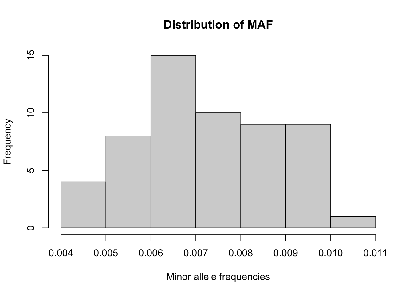
- Run the single variant association tests in PLINK (only for the extracted variants).
cmd <- sprintf("%s --bfile chr1_region_rv --pheno %s/rv_pheno.txt --pheno-name Pheno --glm allow-no-covars  --out test_plink", plink2_binary, files_dir)
system(cmd)
sv_pvals <- fread("test_plink.Pheno.glm.linear")
str(sv_pvals) # what variables are used to store p-values and effect sizes?
Classes 'data.table' and 'data.frame': 56 obs. of 16 variables:
$ #CHROM : int 1 1 1 1 1 1 1 1 1 1 ...
$ POS : int 12030946 12032428 12057950 12095233 12100532 12110879 12121069 12137783 12137898 12143774 ...
$ ID : chr "1:12030946:T:C" "1:12032428:A:C" "1:12057950:C:T" "1:12095233:A:C" ...
$ REF : chr "C" "C" "T" "C" ...
$ ALT : chr "T" "A" "C" "A" ...
$ PROVISIONAL_REF?: chr "Y" "Y" "Y" "Y" ...
$ A1 : chr "T" "A" "C" "A" ...
$ OMITTED : chr "C" "C" "T" "C" ...
$ A1_FREQ : num 0.00498 0.00854 0.00789 0.00593 0.00628 ...
$ TEST : chr "ADD" "ADD" "ADD" "ADD" ...
$ OBS_CT : int 9949 9949 9949 9949 9949 9949 9949 9949 9949 9949 ...
$ BETA : num 0.0557 0.0642 -0.3236 -0.076 -0.1003 ...
$ SE : num 0.1021 0.0773 0.0802 0.0936 0.091 ...
$ T_STAT : num 0.546 0.831 -4.035 -0.812 -1.103 ...
$ P : num 0.585383 0.406254 0.000055 0.416873 0.270211 ...
$ ERRCODE : chr "." "." "." "." ...
- attr(*, ".internal.selfref")=<externalptr> - What would be your significance threshold after applying Bonferroni correction for the multiple tests (assume the nominal significance level is 0.05)? Is anything significant after this correction?
# determine the appropriate significance threshold
bonf_threshold <- 0.05 / length(sv_pvals$P)
bonf_threshold
[1] 0.0008928571sv_pvals[ sv_pvals$P < bonf_threshold, ] #CHROM POS ID REF ALT PROVISIONAL_REF? A1 OMITTED
1: 1 12057950 1:12057950:C:T T C Y C T
2: 1 12183493 1:12183493:G:A A G Y G A
3: 1 12360016 1:12360016:G:A A G Y G A
4: 1 12405413 1:12405413:T:C C T Y T C
5: 1 12639385 1:12639385:G:A A G Y G A
6: 1 12734720 1:12734720:A:C C A Y A C
A1_FREQ TEST OBS_CT BETA SE T_STAT P ERRCODE
1: 0.00789024 ADD 9949 -0.323574 0.0801934 -4.03492 5.50288e-05 .
2: 0.00773947 ADD 9949 0.274311 0.0814842 3.36643 7.64368e-04 .
3: 0.00643281 ADD 9949 -0.310260 0.0898433 -3.45335 5.55975e-04 .
4: 0.00487486 ADD 9949 0.359249 0.1019850 3.52258 4.29282e-04 .
5: 0.00567896 ADD 9949 0.391421 0.0955243 4.09761 4.20759e-05 .
6: 0.00849332 ADD 9949 -0.278236 0.0769709 -3.61482 3.02042e-04 .- Make a volcano plot (i.e. plot log10 p-values against the effect sizes). Which of the Burden/SKAT/ACAT tests do you expect will give us most power?
with(sv_pvals, plot(x=BETA, y=-log10(sv_pvals$P), xlab = "Effect size", ylab = "-log10P")) 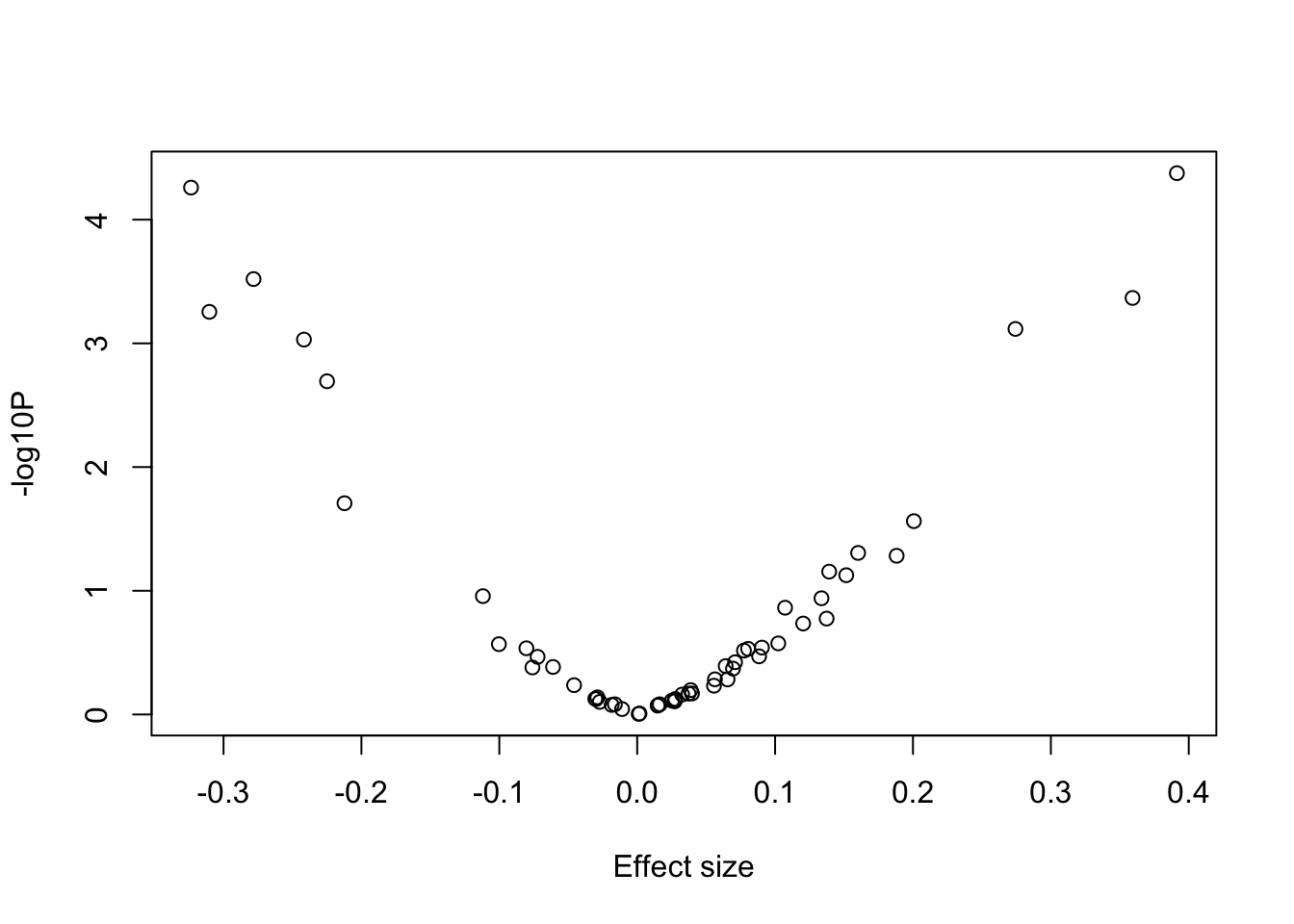
- We will first compare three collapsing/burden approaches:
- CAST (Binary collapsing approach): for each individual, count if they have a rare allele at any of the sites
- MZ Test/GRANVIL (Count based collapsing): for each individual, count the total number of sites where a rare allele is present
- Weighted burden test: for each individual, take a weighted count of
the rare alleles across sites (for the weights, use
weights <- dbeta(MAF, 1, 25))
For each approach, first need to generate the burden scores.
# CAST : count number of rare alleles for each person and determine if it is > 0
sum_alleles_per_sample <- rowSums(G)
burden.cast <- as.numeric( sum_alleles_per_sample > 0 )

# MZ : count number of sites with rare alleles for each person
burden.mz <- rowSums(G > 0)

# Weighted burden : weighted sum of genotype counts across sites
weights <- dbeta(maf, 1, 25)
burden.weighted <- G %*% weights
Run a test for association between the phenotype and each burden
score using the lm() R function, e.g.
# e.g. for CAST
summary(lm(pheno_file$Pheno ~ burden.cast))
Call:
lm(formula = pheno_file$Pheno ~ burden.cast)

Residuals:
    Min      1Q  Median      3Q     Max
-3.9531 -0.6880  0.0012  0.6822  3.6581

Coefficients:
            Estimate Std. Error t value Pr(>|t|)
(Intercept) 0.002423   0.015317   0.158    0.874
burden.cast 0.017757   0.020422   0.870    0.385

Residual standard error: 1.01 on 9947 degrees of freedom
Multiple R-squared:  7.6e-05,   Adjusted R-squared:  -2.452e-05
F-statistic: 0.7561 on 1 and 9947 DF,  p-value: 0.3846
# for MZ
summary(lm(pheno_file$Pheno ~ burden.mz))
Call:
lm(formula = pheno_file$Pheno ~ burden.mz)

Residuals:
    Min      1Q  Median      3Q     Max
-3.9521 -0.6894 -0.0013  0.6805  3.6591

Coefficients:
            Estimate Std. Error t value Pr(>|t|)
(Intercept) 0.001444   0.013700   0.105    0.916
burden.mz   0.013492   0.011346   1.189    0.234

Residual standard error: 1.01 on 9947 degrees of freedom
Multiple R-squared:  0.0001421, Adjusted R-squared:  4.162e-05
F-statistic: 1.414 on 1 and 9947 DF,  p-value: 0.2344
# Weighted burden
summary(lm(pheno_file$Pheno ~ burden.weighted))
Call:
lm(formula = pheno_file$Pheno ~ burden.weighted)

Residuals:
    Min      1Q  Median      3Q     Max
-3.9519 -0.6896 -0.0014  0.6804  3.6593

Coefficients:
                 Estimate Std. Error t value Pr(>|t|)
(Intercept)     0.0012244  0.0136778   0.090    0.929
burden.weighted 0.0006577  0.0005402   1.217    0.223

Residual standard error: 1.01 on 9947 degrees of freedom
Multiple R-squared:  0.000149,  Adjusted R-squared:  4.846e-05
F-statistic: 1.482 on 1 and 9947 DF,  p-value: 0.2235
Looking further at the weighted burden variant weights
# across a wide MAF range
maf_ranges <- seq(.01,.5, length=100)
plot(dbeta(maf_ranges, 1, 25)  ~ maf_ranges, type = "l", xlab = "MAF", ylab = "Variant weights in weighted burden test")
points(weights ~ maf, col = "red", pch = 18)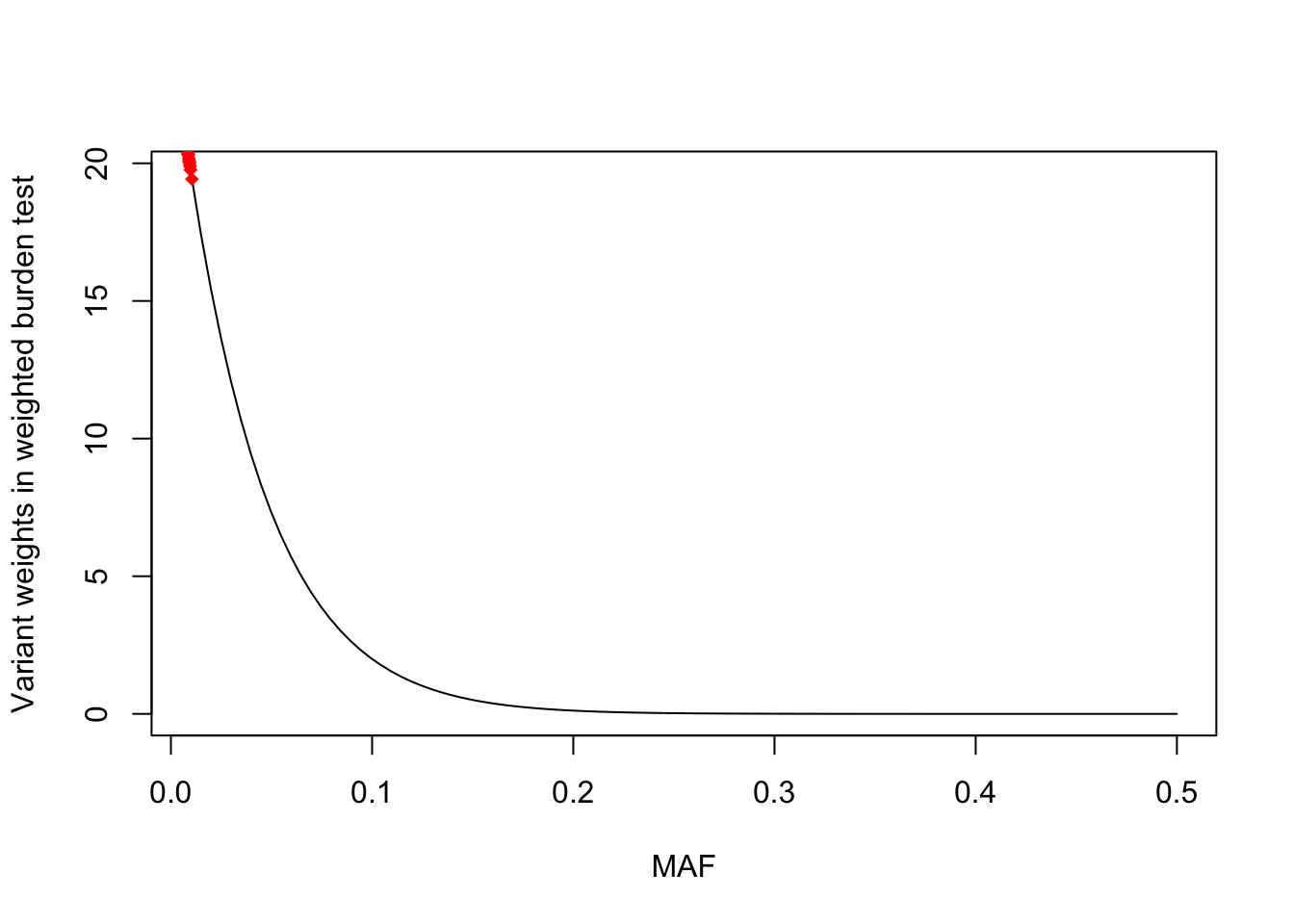
# only looking at variants in the data
plot(weights ~ maf, col = "red", pch = 18, xlab = "MAF", ylab = "Variant weights in weighted burden test")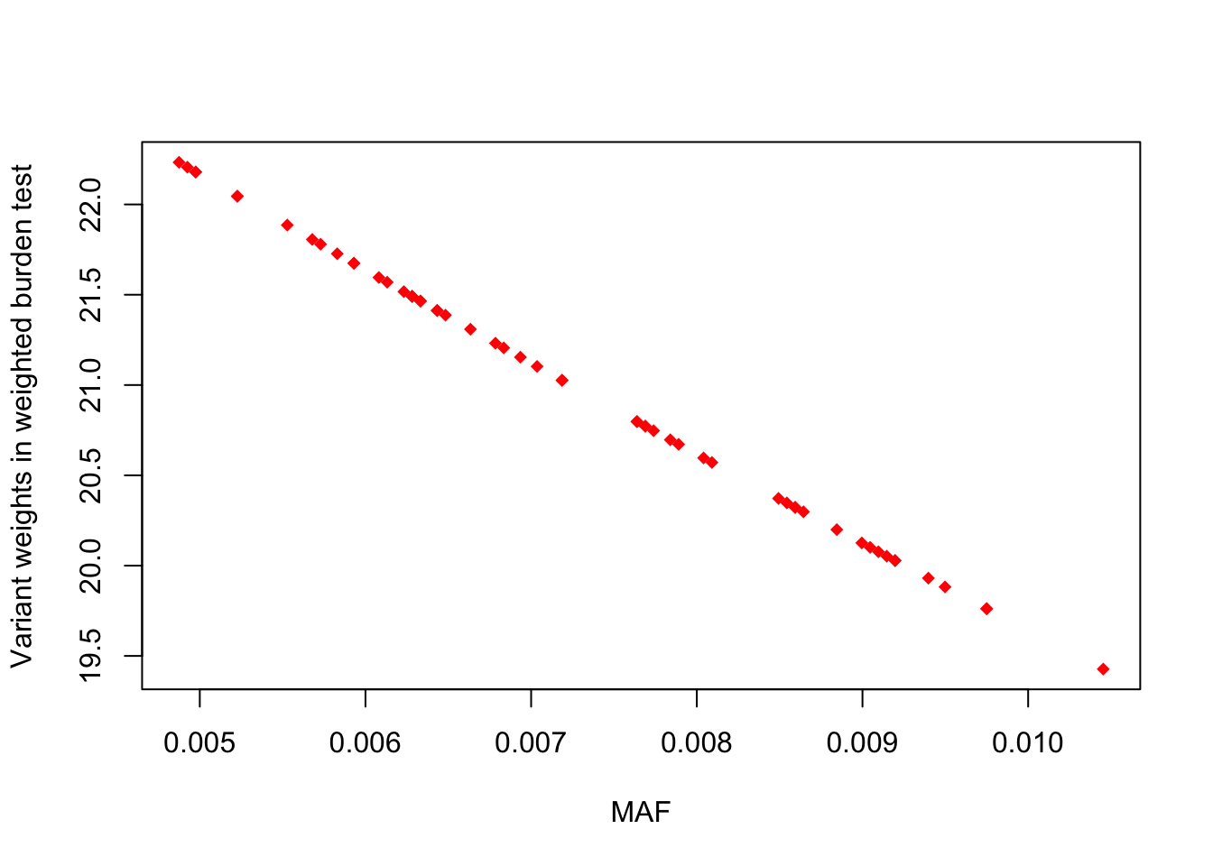
- Now use SKAT to test for an association.
# first fit the null model
skat.null <- SKAT_Null_Model( pheno_file$Pheno ~ 1 , out_type = "C")
# Run SKAT association test (returns a list - p-value is in `$p.value`)
skat_sumstats <- SKAT(G, skat.null )
str(skat_sumstats)
List of 7
$ p.value : num 8.75e-11
$ p.value.resampling: NULL
$ Test.Type : chr "davies"
$ Q : num [1, 1] 4833265
$ param :List of 4
..$ liu_pval : num 8.75e-11
..$ Is_Converged : num 0
..$ n.marker : int 56
..$ n.marker.test: int 56
$ pval.zero.msg : NULL
$ test.snp.mac : Named num [1:56] 99 170 157 118 125 161 126 160 114 125 ...
..- attr(*, "names")= chr [1:56] "1:12030946:T:C" "1:12032428:A:C" "1:12057950:C:T" "1:12095233:A:C" ...
- attr(*, "class")= chr "SKAT_OUT"skat_sumstats$p.value[1] 8.745405e-11- Run the omnibus SKAT, but consider setting \(\rho\) (i.e.
r.corr) to 0 and then 1.
- Compare the results to using the CAST,MZ/GRANVIL and Weighted burden collapsing approaches in Question 5 as well as SKAT in Question 6. What tests do these \(\rho\) values correspond to?
# Example for rho = 0
rho <- 0
skat_sumstats_rho <- SKAT(G, skat.null, r.corr = rho )
skat_sumstats_rho$p.value # = SKAT test
[1] 8.745405e-11rho <- 1
skat_sumstats_rho <- SKAT(G, skat.null, r.corr = rho )
skat_sumstats_rho$p.value # = weighted burden test[1] 0.2234603- Now consider the omnibus version of SKAT, but use the “optimal.adj” approach which searches across a range of rho values.
# Run SKATO association test using grid of rho values
skat_sumstats_rho_grid <- SKAT(G, skat.null, method="optimal.adj")
skat_sumstats_rho_grid$p.value
[1] 6.121784e-10- Run ACATV on the single variant p-values. The basic command would look like
# `weights` vector is from Question 5
acat.weights <- weights * weights * maf * (1 - maf)
ACAT(sv_pvals$P, weights = acat.weights)
[1] 0.00112117- Run ACATO combining the SKAT and BURDEN p-values (from Question 7) with the ACATV p-value (from Question 9).
# Fill in the p-values
SKAT_pvalue <- 8.745405e-11
Burden_pvalue <- 0.2234603
ACATV_pvalue <- 0.00112117
# compute ACATO
ACAT( c(SKAT_pvalue, Burden_pvalue, ACATV_pvalue) )
[1] 2.623621e-10Extra
You can explore the impact of different genetic architectures by analyzing 3 simulated phenotypes in “data/rv_pheno_extended.txt”. More specifically, you can run the same analyses done above for each of these traits and compare the performance of the tests relative to how variant effects were simulated:
- “Pheno_sparse”: a single causal variant (i.e. sparse genetic architecture)
- “Pheno_burden_skat”: 60% of the variant are causal, and they all have positive effects on the trait
- “Pheno_skat”: 20% of the variants are causal and the effect direction (+/-) is randomly assigned
Here is R code used to generate the phenotypes:
G <- BEDMatrix::BEDMatrix("data/rv_geno_chr1", simple_names = TRUE)
N <- nrow(G)
nsnps <- ncol(G)

# Parameters to change
# sparse : set n.causal = 1
# burden_skat : set prop_causal=0.6 and prop_pos_beta=1
# skat : set prop_causal=0.2 and prop_pos_beta=0.5
prop_causal <- 1
prop_pos_beta <- 1
h2g <- 0.01

n.causal <- round(nsnps * prop_causal)
causal.index <- sample(ncol(G), n.causal)

b_snp <- sqrt(h2g/n.causal)
beta <- rep(b_snp, n.causal)
beta_sign <- sample(c(rep(1, round(n.causal * prop_pos_beta)), rep(-1, n.causal - round(n.causal * prop_pos_beta))))
h2e <- 1 - h2g

y <- scale(G[, causal.index]) %*% beta + rnorm(N, sd = sqrt(h2e))
sessionInfo()R version 4.3.0 (2023-04-21)
Platform: aarch64-apple-darwin20 (64-bit)
Running under: macOS 14.7.4
Matrix products: default
BLAS: /Library/Frameworks/R.framework/Versions/4.3-arm64/Resources/lib/libRblas.0.dylib
LAPACK: /Library/Frameworks/R.framework/Versions/4.3-arm64/Resources/lib/libRlapack.dylib; LAPACK version 3.11.0
locale:
[1] en_US.UTF-8/en_US.UTF-8/en_US.UTF-8/C/en_US.UTF-8/en_US.UTF-8
time zone: America/Chicago
tzcode source: internal
attached base packages:
[1] stats graphics grDevices utils datasets methods base
other attached packages:
[1] ggplot2_3.4.2 ACAT_0.91 SKAT_2.2.5 RSpectra_0.16-1
[5] SPAtest_3.1.2 Matrix_1.5-4 BEDMatrix_2.0.3 dplyr_1.1.2
[9] data.table_1.14.8
loaded via a namespace (and not attached):
[1] sass_0.4.6 utf8_1.2.3 generics_0.1.3 stringi_1.7.12
[5] lattice_0.21-8 digest_0.6.31 magrittr_2.0.3 evaluate_0.21
[9] grid_4.3.0 fastmap_1.1.1 rprojroot_2.0.3 workflowr_1.7.0
[13] jsonlite_1.8.5 promises_1.2.0.1 fansi_1.0.4 scales_1.2.1
[17] jquerylib_0.1.4 cli_3.6.1 rlang_1.1.1 munsell_0.5.0
[21] withr_2.5.0 cachem_1.0.8 yaml_2.3.7 tools_4.3.0
[25] colorspace_2.1-0 httpuv_1.6.11 crochet_2.3.0 vctrs_0.6.2
[29] R6_2.5.1 lifecycle_1.0.3 git2r_0.32.0 stringr_1.5.0
[33] fs_1.6.2 pkgconfig_2.0.3 pillar_1.9.0 bslib_0.5.0
[37] later_1.3.1 gtable_0.3.3 glue_1.6.2 Rcpp_1.0.10
[41] highr_0.10 xfun_0.39 tibble_3.2.1 tidyselect_1.2.0
[45] rstudioapi_0.14 knitr_1.43 htmltools_0.5.5 rmarkdown_2.22
[49] compiler_4.3.0