Solution for Practical 5: Conditional and Joint Analysis (COJO)
Summer Institute of Statical Genetics (Module 15)
2023-07-25
Last updated: 2025-06-01
Checks: 6 1
Knit directory:
SISG2025_Association_Mapping/
This reproducible R Markdown analysis was created with workflowr (version 1.7.0). The Checks tab describes the reproducibility checks that were applied when the results were created. The Past versions tab lists the development history.
The R Markdown is untracked by Git. To know which version of the R
Markdown file created these results, you’ll want to first commit it to
the Git repo. If you’re still working on the analysis, you can ignore
this warning. When you’re finished, you can run
wflow_publish to commit the R Markdown file and build the
HTML.
Great job! The global environment was empty. Objects defined in the global environment can affect the analysis in your R Markdown file in unknown ways. For reproduciblity it’s best to always run the code in an empty environment.
The command set.seed(20230530) was run prior to running
the code in the R Markdown file. Setting a seed ensures that any results
that rely on randomness, e.g. subsampling or permutations, are
reproducible.
Great job! Recording the operating system, R version, and package versions is critical for reproducibility.
Nice! There were no cached chunks for this analysis, so you can be confident that you successfully produced the results during this run.
Great job! Using relative paths to the files within your workflowr project makes it easier to run your code on other machines.
Great! You are using Git for version control. Tracking code development and connecting the code version to the results is critical for reproducibility.
The results in this page were generated with repository version 421fcd0. See the Past versions tab to see a history of the changes made to the R Markdown and HTML files.
Note that you need to be careful to ensure that all relevant files for
the analysis have been committed to Git prior to generating the results
(you can use wflow_publish or
wflow_git_commit). workflowr only checks the R Markdown
file, but you know if there are other scripts or data files that it
depends on. Below is the status of the Git repository when the results
were generated:
Ignored files:
    Ignored:    .DS_Store
    Ignored:    .qodo/
    Ignored:    analysis/.DS_Store
    Ignored:    data/run_regenie.r
    Ignored:    data/sim_rels_geno.bed
    Ignored:    exe/
    Ignored:    ldRef.log
    Ignored:    lectures/
    Ignored:    mk_website.R
    Ignored:    notes.txt
    Ignored:    tmp/

Untracked files:
    Untracked:  .mk_website.R.swp
    Untracked:  GWAS.ma
    Untracked:  _workflowr.yml
    Untracked:  analysis/.QG3_Downstream-Analyses_practical_Key.Rmd.swp
    Untracked:  analysis/.index.Rmd.swp
    Untracked:  analysis/QG3_Association_Testing_practical_Key.Rmd
    Untracked:  analysis/QG3_Beyond_Standard_GWAS_practical_Key.Rmd
    Untracked:  analysis/QG3_CC_Imbalance_practical_Key.Rmd
    Untracked:  analysis/QG3_Downstream-Analyses_practical_Key.Rmd
    Untracked:  analysis/QG3_Plink_Population_Structure_practical_Key.Rmd
    Untracked:  analysis/QG3_Polygenic_Scores_practical_Key.Rmd
    Untracked:  analysis/QG3_Power-Design_practical_Key.Rmd
    Untracked:  analysis/QG3_RV_tests_practical_Key.Rmd
    Untracked:  analysis/QG3_Relatedness_REGENIE_practical_Key.Rmd
    Untracked:  analysis/figure/
    Untracked:  causals.snplist
    Untracked:  ldRef.bed
    Untracked:  ldRef.bim
    Untracked:  ldRef.fam
    Untracked:  ldRef.map
    Untracked:  ldRef.ped
    Untracked:  sim.config

Unstaged changes:
    Modified:   analysis/QG3_Downstream-Analyses_practical.Rmd
    Modified:   analysis/_site.yml
Note that any generated files, e.g. HTML, png, CSS, etc., are not included in this status report because it is ok for generated content to have uncommitted changes.
There are no past versions. Publish this analysis with
wflow_publish() to start tracking its development.
This practical runs on the SISG2023 server.
This practical aims at
Familiarizing you with GCTA-COJO (or COJO in short)
Exploring different factors influencing COJO outcomes
The practical is run in R but uses the R
function system() to run PLINK and
GCTA from the terminal. If you have PLINK and
GCTA installed on your own computer then you could also run
it locally if your prefer. In that case you’d need to update a few links
provided below.
The COJO algorithm is not designed for fine-mapping per se. However, many of the challenges illustrated and discussed in this practical are relevant for any method using external linkage disequilibrium (LD) reference.
Part I: the data
We provide an R code that simulates a 1 Mb long
chromosome with M=2000 SNPs organized within 20 LD blocks.
Each block contains 100 SNPs, among which 5 causal variants. SNPs within
a block are numbered between 1 and 100, such that the squared
correlation \(r^2_{i_{k}j_{k}}\) of
allele counts at SNP \(i_k\) and \(j_k\) within LD block \(k\) is
\[ r^2_{i_{k}j_{k}} = \rho_k^{2|i_k-j_k|} \]
LD blocks are characterized by the parameters \(\rho^2_k\), which varies from 0.1 (when \(k=1\); low LD locus) to 0.9 (when \(k=20\); high LD locus).
The code below generates the LD correlation structure between SNPs in each block.
Run the following commands
set.seed(28072022)
nblocks <- 20
rhos    <- sqrt(seq(0.1,0.9,len=nblocks))
m       <- 100 # number of SNPs per LD block
mcBlock <- 5   # number of causals LD per block
M       <- m * nblocks
R       <- matrix(0,nrow=M,ncol=M)
icausal <- c()
for(k in 1:nblocks){
  l <- ((k-1)*m + 1):(k*m);
  R[l,l]  <- outer(1:m,1:m,FUN=function(i,j) rhos[k]^abs(i-j))
  icausal <- c(icausal,sample(l,mcBlock))
}
The figure code and figure below shows the LD correlation matrix for SNPs the 20-th LD block (\(\rho^2_{20}=0.9\))
k=20
l=((k-1)*m + 1):(k*m)
heatmap(R[l,l],Rowv=NA,Colv=NA)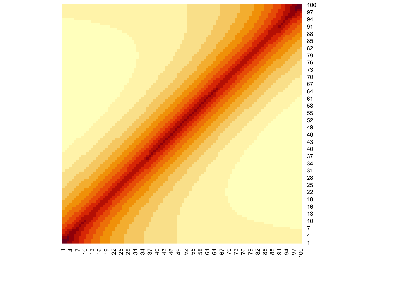
print("Extract of LD structure for 20-th LD block")[1] "Extract of LD structure for 20-th LD block"print( R[l,l][1:5,1:5] ) [,1] [,2] [,3] [,4] [,5]
[1,] 1.0000000 0.9486833 0.9000000 0.8538150 0.8100000
[2,] 0.9486833 1.0000000 0.9486833 0.9000000 0.8538150
[3,] 0.9000000 0.9486833 1.0000000 0.9486833 0.9000000
[4,] 0.8538150 0.9000000 0.9486833 1.0000000 0.9486833
[5,] 0.8100000 0.8538150 0.9000000 0.9486833 1.0000000Run the following commands
chr     <- 10 # Chromosome number
pos     <- 1234557 + sort(sample(0:1e6,M)) # Random Position for SNPs
a1a2    <- do.call("rbind",lapply(1:M,function(j) sample(c("A","C","G","T"),2))) # alleles
snps    <- paste0("SNP",1:M) # SNP ID
ldblock <- rep(1:nblocks,each=m) # LD block ID
names(ldblock) <- snps
The R code below generates and shows the LD score of
each SNP on the chromosome (x-axis: genomic position in Mb; y-axis: LD
score)
Cols <- sample(colors(),nblocks)
ldscores <- diag(crossprod(R))
plot(pos/1e6,ldscores,pch=19,col=Cols[ldblock],
     axes=FALSE,xlab="Genomic Position (Mb)",
     ylab="LD scores")
axis(1);axis(2)
legend("topleft",legend=paste0("Block #",1:nblocks),
       box.lty=0,pch=19,cex=0.5,col=Cols)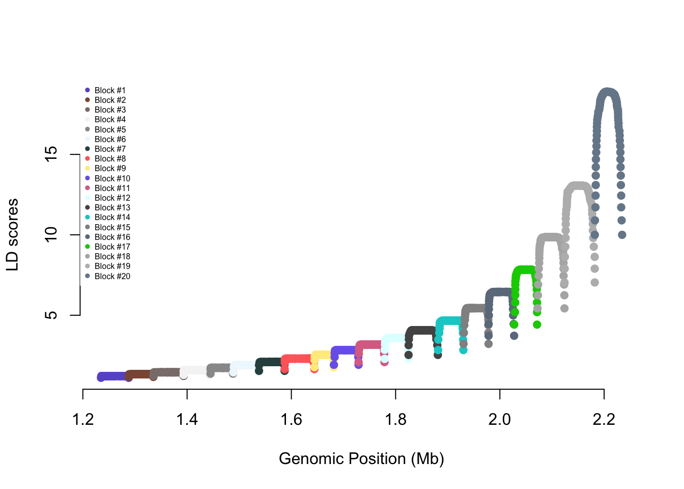
cat(paste0("mean LD score = ",round(mean(ldscores),3),
           " - SD LD score = ",round(sd(ldscores),3)))
mean LD score = 4.598 - SD LD score = 4.13Run the following commands. This is a function to generate genotypes corresponding to the specified LD structure. For simplicity, we simulate all SNPs with an allele frequency equal to 0.5.
library(MASS)
simGeno <- function(R,n){
  z1 <- do.call("cbind",lapply(1:nblocks,function(i){
    l <- ((i-1)*m + 1):(i*m)
    mvrnorm(n=n,mu=rep(0,m),Sigma = R[l,l])
  }))
  z2 <- do.call("cbind",lapply(1:nblocks,function(i){
    l <- ((i-1)*m + 1):(i*m)
    mvrnorm(n=n,mu=rep(0,m),Sigma = R[l,l])
  }))
  x <- (z1>0) + (z2>0)
  return(x)
}
Run the following commands to genarate genotypes and
phenotypes of GWAS participants. GWAS sample size is
Ngwas=100000
Ngwas <- 5e4

## Simulate genotypes
Xgwas <- simGeno(n = Ngwas,R)

## Simulate phenotype
mc    <- length(icausal) # total number of causal variants
q2    <- 0.01 #variance explained by all SNPs on the chromosome
b     <- rnorm(n=mc,mean=0,sd=sqrt(q2/mc))
g     <- sqrt(2)*c((Xgwas[,icausal]-1)%*%b)
e     <- rnorm(n=Ngwas,mean=0,sd=sqrt(1-q2))
Ygwas <- g + e

## Running GWAS
var_x <- apply(Xgwas,2,var)
beta  <- cov(Xgwas,Ygwas) / var_x # estimated regression coefficients
se    <- sqrt( (var(Ygwas) - beta*beta*var_x)/((Ngwas-2)*var_x) ) # standard errors
pval  <- 2 * pt(q=abs(beta/se),df=Ngwas-2,lower.tail = F) # T-distribution

## GWAS data - COJO format
gwas  <- cbind.data.frame(SNP=snps,A1=a1a2[,1],A2=a1a2[,2],
                          Freq=colMeans(Xgwas)/2,beta=beta,
                          se=se,P=pval,N=Ngwas)
print(head(gwas,3))
SNP A1 A2 Freq beta se P N
1 SNP1 C T 0.49842 -0.008869039 0.006329104 0.1611275 50000
2 SNP2 T C 0.49813 -0.001241079 0.006325583 0.8444544 50000
3 SNP3 C A 0.50211 0.008500874 0.006342246 0.1801354 50000# folder where to store the data
# default is ".", i.e. current directory
# this can be changed
datPath <- "."
write.table(gwas,paste0(datPath,"/GWAS.ma"),
quote=FALSE,row.names=FALSE,
col.names=TRUE,sep="\t")
causals <- snps[icausal]
write(causals,paste0(datPath,"/causals.snplist")) ## list of causal SNPsRun the following commands to simulate a LD reference (i.e.,
set of genotypes in PLINK format) from the same
population.
## Set path for PLINK
plink   <- "exe/plink"

## Simulate and write LD ref
simLDref <- function(Nldref){
  Xldref <- simGeno(n = Nldref,R)
  refGeno <- t(sapply(1:M,function(j) {
    c(paste0(a1a2[j,1],"\t",a1a2[j,1]),
      paste0(a1a2[j,1],"\t",a1a2[j,2]),
      paste0(a1a2[j,2],"\t",a1a2[j,2]))
  }))
  ped <- do.call("cbind",lapply(1:M,function(j){
    refGeno[j,1+Xldref[,j]]}
  ))
  ## fam file
  iid    <- paste0("IID",1:Nldref)
  fid    <- iid
  pid    <- rep(0,Nldref)
  mid    <- rep(0,Nldref)
  sex    <- sample(1:2,Nldref,replace=TRUE)
  pheno  <- rep(-9,Nldref)
  fam    <- cbind.data.frame(fid,iid,pid,mid,sex,pheno)

  ## ped/geno
  mapData <- cbind.data.frame(chr,snps,0,pos)
  pedData <- cbind.data.frame(fam,ped)

  write.table(mapData,paste0(datPath,"/ldRef.map"),
              quote=FALSE,row.names=FALSE,col.names=FALSE,sep="\t")
  write.table(pedData,paste0(datPath,"/ldRef.ped"),
              quote=FALSE,row.names=FALSE,col.names=FALSE,sep="\t")
  system(paste0(plink," --file ldRef --make-bed --out ldRef"))
}
simLDref(Nldref = 5000)
Part II: running COJO
If you have run all the commands above then the following files must be available in your current directory. To check type the following command in the terminal.
ls -lt GWAS.ma
ls -lt ldRef.*
-rw-r--r-- 1 joelle.mbatchou staff 167356 Jun 1 10:02 GWAS.ma
-rw-r--r-- 1 joelle.mbatchou staff 1045 Jun 1 10:02 ldRef.log
-rw-r--r-- 1 joelle.mbatchou staff 48893 Jun 1 10:02 ldRef.bim
-rw-r--r-- 1 joelle.mbatchou staff 122786 Jun 1 10:02 ldRef.fam
-rw-r--r-- 1 joelle.mbatchou staff 2500003 Jun 1 10:02 ldRef.bed
-rw-r--r-- 1 joelle.mbatchou staff 40122786 Jun 1 10:02 ldRef.ped
-rw-r--r-- 1 joelle.mbatchou staff 40893 Jun 1 10:02 ldRef.mapYou can now run COJO. Either from the terminal
GCTA=exe/gcta64_v1.94
${GCTA} --bfile ldRef --cojo-file GWAS.ma --chr 10 --cojo-slct --cojo-p 2.5e-5 --out test1
*******************************************************************
* Genome-wide Complex Trait Analysis (GCTA)
* version v1.94.1 Mac
* (C) 2010-present, Yang Lab, Westlake University
* Please report bugs to Jian Yang <jian.yang@westlake.edu.cn>
*******************************************************************
Analysis started at 10:02:17 CDT on Sun Jun 01 2025.
Hostname: R1YG04N9NV
Accepted options:
--bfile ldRef
--cojo-file GWAS.ma
--chr 10
--cojo-slct
--cojo-p 2.5e-05
--out test1
Reading PLINK FAM file from [ldRef.fam].
5000 individuals to be included from [ldRef.fam].
Reading PLINK BIM file from [ldRef.bim].
2000 SNPs to be included from [ldRef.bim].
2000 SNPs on chromosome 10 are included in the analysis.
Reading PLINK BED file from [ldRef.bed] in SNP-major format ...
Genotype data for 5000 individuals and 2000 SNPs to be included from [ldRef.bed].
Reading GWAS summary-level statistics from [GWAS.ma] ...
GWAS summary statistics of 2000 SNPs read from [GWAS.ma].
Phenotypic variance estimated from summary statistics of all 2000 SNPs: 1.00111 (variance of logit for case-control studies).
Matching the GWAS meta-analysis results to the genotype data ...
Calculating allele frequencies ...
2000 SNPs are matched to the genotype data.
Calculating the variance of SNP genotypes ...
Performing stepwise model selection on 2000 SNPs to select association signals ... (p cutoff = 2.5e-05; collinearity cutoff = 0.9)
(Assuming complete linkage equilibrium between SNPs which are more than 10Mb away from each other)
5 associated SNPs have been selected.
10 associated SNPs have been selected.
Finally, 11 associated SNPs are selected.
Performing joint analysis on all the 11 selected signals ...
Saving the 11 independent signals to [test1.jma.cojo] ...
Saving the LD structure of 11 independent signals to [test1.ldr.cojo] ...
Saving the conditional analysis results of 1989 remaining SNPs to [test1.cma.cojo] ...
(0 SNPs eliminated by backward selection and 0 SNPs filtered by collinearity test are not included in the output)
Analysis finished at 10:02:18 CDT on Sun Jun 01 2025
Overall computational time: 1.61 sec.or from R (calling terminal using the
system() command)
gcta <- "exe/gcta64_v1.94"

system(paste0(gcta," --bfile ldRef ",
              "--cojo-file GWAS.ma --chr 10 ",
              "--cojo-slct --cojo-p 2.5e-5 --out test1"))
Question 1. How many SNPs are detected? How many of those are
causal SNPs? (Note that you can obtain causal SNPs in your currrent
R session as causals = snps[icausal], or in
the file named causals.snplist).
The number of SNPs detected by COJO is displayed in the log file “Saving the 10 independent signals to [test1.jma.cojo].” and corresponds to the number of rows (minus one) in the *.jma.cojo file. Here, 10 SNPs were detected…
cojo1 <- read.table("test1.jma.cojo",h=T,stringsAsFactors = FALSE) ## Read COJO results
print( table(cojo1$SNP%in%snps[icausal]) ) ## Count how many are causal
FALSE  TRUE
    2     9
…including 10 causal variants.
Question 2. Regenerate LD reference data with a lower sample
size Nldref=2000, 1000 and 500 and rerun 1). What do you
observe? Are all LD blocks affected the same?
Let us focus on the smallest LD reference
Nldref=2000. We modify and re-run some of the
R commands given above…
simLDref(Nldref = 500)
system(paste0(gcta," --bfile ldRef ",
              "--cojo-file GWAS.ma --chr 10 ",
              "--cojo-slct --cojo-p 2.5e-5 --out test2"))
cojo2 <- read.table("test2.jma.cojo",h=T,stringsAsFactors = FALSE) ## Read COJO results
print( table(cojo2$SNP%in%snps[icausal]) ) ## Count how many are causal
FALSE  TRUE
  227    21
We can see that 246 SNPs are now detected but only 23 of them are causal. To see if all LD blocks are affected the same, we can visualize the number of COJO SNPs (here mostly false positives) in each LD block using (for example) the following command.
barplot(table(ldblock[cojo2$SNP]),ylab="# COJO SNPs in each LD block",
        xlab="LD blocks (1: low LD; 20: high LD)")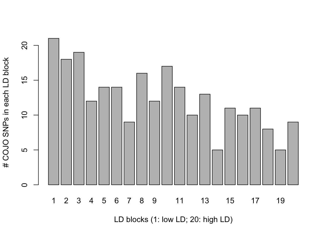
Conclusion: the inflation is larger in low LD blocks.
Question 3. Set the variance explained by SNPs on the chromosome to 3% (q2=0.03) and re-run 1) and 2). What can you conclude regarding the number of SNPs detected and the proportion of non-causal SNPs detected?
Conclusion: the inflation of false positives observed with small LD reference is larger when the signal (\(q^2\)) is strong.
Part III: fixing COJO?
There is no simple way to fix the inflation of false positive observed when the LD reference is too small. As a rule of thumb, Yang et al. (GCTA website) recommend using sample sizes of at least 4000. Nevertheless, we observe that using a more stringent threshold for detecting collinearity might help.
Question 4. Set the variance explained by SNPs on the
chromosome to 3% (q2=0.03) and the size of the LD reference to 1000.
Re-run COJO adding the following flag --cojo-collinear 0.1.
Quantify the improvement in the number of false positives.
q2    <- 0.03 #variance explained by all SNPs on the chromosome
b     <- rnorm(n=mc,mean=0,sd=sqrt(q2/mc))
g     <- sqrt(2)*c((Xgwas[,icausal]-1)%*%b)
e     <- rnorm(n=Ngwas,mean=0,sd=sqrt(1-q2))
Ygwas <- g + e
beta  <- cov(Xgwas,Ygwas) / var_x # estimated regression coefficients
se    <- sqrt( (var(Ygwas) - beta*beta*var_x)/((Ngwas-2)*var_x) ) # standard errors
pval  <- 2 * pt(q=abs(beta/se),df=Ngwas-2,lower.tail = F) # T-distribution
gwas  <- cbind.data.frame(SNP=snps,A1=a1a2[,1],A2=a1a2[,2],
                          Freq=colMeans(Xgwas)/2,beta=beta,
                          se=se,P=pval,N=Ngwas)
print(head(gwas,3))
SNP A1 A2 Freq beta se P N
1 SNP1 C T 0.49842 0.0029933730 0.006325153 0.6360375 50000
2 SNP2 T C 0.49813 -0.0005899297 0.006321526 0.9256491 50000
3 SNP3 C A 0.50211 -0.0077559916 0.006338196 0.2210747 50000write.table(gwas,paste0(datPath,"/GWAS.ma"),
quote=FALSE,row.names=FALSE,
col.names=TRUE,sep="\t")
## Simulate LD reference and run COJO
simLDref(Nldref = 1000)
system(paste0(gcta," --bfile ldRef ",
"--cojo-file GWAS.ma --chr 10 ",
"--cojo-slct --cojo-p 2.5e-5 --out test3"))
cojo3 <- read.table("test3.jma.cojo",h=T,stringsAsFactors = FALSE)
print( table(cojo3$SNP%in%snps[icausal]) ) ## Count how many are causal
FALSE  TRUE
  584    45
system(paste0(gcta," --bfile ldRef ",
"--cojo-file GWAS.ma --chr 10 --cojo-collinear 0.05 ",
"--cojo-slct --cojo-p 2.5e-5 --out test4"))
cojo4 <- read.table("test4.jma.cojo",h=T,stringsAsFactors = FALSE)
print( table(cojo4$SNP%in%snps[icausal]) ) ## Count how many are causal
FALSE  TRUE
    8    24
Conclusion: using a more stringent collinearity threshold can reduce the proportion of false positives.
sessionInfo()R version 4.3.0 (2023-04-21)
Platform: aarch64-apple-darwin20 (64-bit)
Running under: macOS 14.7.4
Matrix products: default
BLAS: /Library/Frameworks/R.framework/Versions/4.3-arm64/Resources/lib/libRblas.0.dylib
LAPACK: /Library/Frameworks/R.framework/Versions/4.3-arm64/Resources/lib/libRlapack.dylib; LAPACK version 3.11.0
locale:
[1] en_US.UTF-8/en_US.UTF-8/en_US.UTF-8/C/en_US.UTF-8/en_US.UTF-8
time zone: America/Chicago
tzcode source: internal
attached base packages:
[1] stats graphics grDevices utils datasets methods base
other attached packages:
[1] MASS_7.3-58.4
loaded via a namespace (and not attached):
[1] vctrs_0.6.2 cli_3.6.1 knitr_1.43 rlang_1.1.1
[5] xfun_0.39 highr_0.10 stringi_1.7.12 promises_1.2.0.1
[9] jsonlite_1.8.5 workflowr_1.7.0 glue_1.6.2 rprojroot_2.0.3
[13] git2r_0.32.0 htmltools_0.5.5 httpuv_1.6.11 sass_0.4.6
[17] fansi_1.0.4 rmarkdown_2.22 evaluate_0.21 jquerylib_0.1.4
[21] tibble_3.2.1 fastmap_1.1.1 yaml_2.3.7 lifecycle_1.0.3
[25] stringr_1.5.0 compiler_4.3.0 fs_1.6.2 Rcpp_1.0.10
[29] pkgconfig_2.0.3 rstudioapi_0.14 later_1.3.1 digest_0.6.31
[33] R6_2.5.1 utf8_1.2.3 pillar_1.9.0 magrittr_2.0.3
[37] bslib_0.5.0 tools_4.3.0 cachem_1.0.8