Interaction testing and vQTL mapping

Last updated: 2025-06-10

Checks: 6 1

Knit directory: SISG2025_Association_Mapping/

This reproducible R Markdown analysis was created with workflowr (version 1.7.0). The Checks tab describes the reproducibility checks that were applied when the results were created. The Past versions tab lists the development history.

R Markdown file: uncommitted changes

The R Markdown is ignored by Git. To know which version of the R Markdown file created these results, you’ll want to first commit it to the Git repo. If you’re still working on the analysis, you can ignore this warning. When you’re finished, you can run wflow_publish to commit the R Markdown file and build the HTML.

Environment: empty

Great job! The global environment was empty. Objects defined in the global environment can affect the analysis in your R Markdown file in unknown ways. For reproduciblity it’s best to always run the code in an empty environment.

Seed: set.seed(20230530)

The command set.seed(20230530) was run prior to running the code in the R Markdown file. Setting a seed ensures that any results that rely on randomness, e.g. subsampling or permutations, are reproducible.

Session information: recorded

Great job! Recording the operating system, R version, and package versions is critical for reproducibility.

Cache: none

Nice! There were no cached chunks for this analysis, so you can be confident that you successfully produced the results during this run.

File paths: relative

Great job! Using relative paths to the files within your workflowr project makes it easier to run your code on other machines.

Repository version: e43c815

Great! You are using Git for version control. Tracking code development and connecting the code version to the results is critical for reproducibility.

The results in this page were generated with repository version e43c815. See the Past versions tab to see a history of the changes made to the R Markdown and HTML files.

Note that you need to be careful to ensure that all relevant files for the analysis have been committed to Git prior to generating the results (you can use wflow_publish or wflow_git_commit). workflowr only checks the R Markdown file, but you know if there are other scripts or data files that it depends on. Below is the status of the Git repository when the results were generated:


Ignored files:
    Ignored:    .DS_Store
    Ignored:    .qodo/
    Ignored:    analysis/.DS_Store
    Ignored:    analysis/QG3_Association_Testing_practical_Key.Rmd
    Ignored:    analysis/QG3_Beyond_Standard_GWAS_practical_Key.Rmd
    Ignored:    analysis/QG3_CC_Imbalance_practical_Key.Rmd
    Ignored:    analysis/QG3_Downstream-Analyses_practical_Key.Rmd
    Ignored:    analysis/QG3_Plink_Population_Structure_practical_Key.Rmd
    Ignored:    analysis/QG3_Polygenic_Scores_practical_Key.Rmd
    Ignored:    analysis/QG3_Power-Design_practical_Key.Rmd
    Ignored:    analysis/QG3_RV_tests_practical_Key.Rmd
    Ignored:    analysis/QG3_Relatedness_REGENIE_practical_Key.Rmd
    Ignored:    data/run_regenie.r
    Ignored:    data/sim_rels_geno.bed
    Ignored:    exe/
    Ignored:    lectures/
    Ignored:    mk_website.R
    Ignored:    notes.txt
    Ignored:    tmp/

Untracked files:
    Untracked:  .mk_website.R.swp
    Untracked:  _workflowr.yml
    Untracked:  analysis/.Rhistory
    Untracked:  analysis/.index.Rmd.swp
    Untracked:  analysis/QG3_Plink_Population_Structure_practical_Key_cache/

Unstaged changes:
    Modified:   analysis/QG3_Beyond_Standard_GWAS_practical.Rmd

Note that any generated files, e.g. HTML, png, CSS, etc., are not included in this status report because it is ok for generated content to have uncommitted changes.

These are the previous versions of the repository in which changes were made to the R Markdown (analysis/QG3_Beyond_Standard_GWAS_practical_Key.Rmd) and HTML (docs/QG3_Beyond_Standard_GWAS_practical_Key.html) files. If you’ve configured a remote Git repository (see ?wflow_git_remote), click on the hyperlinks in the table below to view the files as they were in that past version.

File	Version	Author	Date	Message
html	5949e8a	Joelle Mbatchou	2025-06-10	Build site.

Before you begin:

Make sure that R is installed on your computer For this lab, we will use the following R libraries:

library(qqman)

This practical aims at illustrating the relationship between tests for vQTLs and tests for interaction effects. We provide a set of R commands below to simulate the phenotypes, genotypes and covariates (at \(M=1000\) SNPs) of \(N=10,000\) samples and 2 covariates. We will chose the first of the 10 SNPs to be causal (either QTL, vQTL or both). We generate two phenotypes which differ based on whether the causal variant influences the phenotypic variance of the trait directly or influences the phenotypic mean through GxE effects.

\[ E(Y_{vQTL}) = G\beta,\; Var(Y_{vQTL}) = 1 + G\alpha \]

\[ E(Y_{gxe}) = G\beta + E\gamma + (G\times E)\alpha \]

Simulated dataset

Copy/Run the following command to enable the simulate_vqtl_data function in your current R environment.

set.seed(646909) # For reproducibility
n_individuals <- 10000
n_snps <- 1000

# Function to simulate genotype, phenotype, and covariate data
# Mean effect != 0 corresponds to QTL
# Variance effect != 0 corresponds to vQTL
simulate_vqtl_data <- function(n_individuals = 10000, n_snps = 1000, mean_effect = 1, variance_effect = 2) {

  # Simulate genotype data with no LD (0, 1, 2 for SNPs)
  genotype_data <- as.data.frame(matrix(sample(0:2, n_individuals * n_snps, replace = TRUE), 
                                        nrow = n_individuals, ncol = n_snps))
  colnames(genotype_data) <- paste0("SNP", 1:n_snps)

  # Simulate environmental covariate (e.g., smoking status)
  covariate_data <- data.frame(
    environment = factor(sample(c("non-smoker", "smoker"), n_individuals, replace = TRUE), levels = c("non-smoker", "smoker")),
    age = runif(n_individuals, 40,60)
  )

  # Approach 1: Modeling SNP effect in the phenotypic variance
  phenotype_variance <- rnorm(n_individuals, 
                              mean = mean_effect * genotype_data$SNP1, 
                              sd = 1 + variance_effect * genotype_data$SNP1)

  # Approach 2: Modeling GxE effect in the phenotypic mean
  phenotype_gxe <- rnorm(n_individuals, 
                         mean = mean_effect * genotype_data$SNP1 + 
                                variance_effect * as.numeric(covariate_data$environment) *genotype_data$SNP1, 
                         sd = 1)

  # Combine phenotypes into a data frame
  phenotype_data <- data.frame(Y_vQTL = phenotype_variance, Y_gxe = phenotype_gxe)

  # Return a list of data frames
  return(list(genotype = genotype_data, phenotype = phenotype_data, covariate = covariate_data))

}

The simulate_vqtl_data function has 4 input parameters: n_individuals (sample size), n_snps (number of SNPs tested), mean_effect (the effect size of the causal variant on the phenotypic mean), variance_effect (the effect size of the causal variant on the phenotypic variance for phenotype Y1 OR the size of the GxE interaction effect for phenotype Y2).

Let’s run a first data set where the causal variant has no effect on the trait, i.e., mean_effect = 0 and variance_effect = 0.

simulated_data <- simulate_vqtl_data(mean_effect = 0, variance_effect = 0)

Note: you can use str(simulated_data) to see a snipper of what’s returned by the simulate_vqtl_data function.

We can visualize the phenotype distribution across genotype groups for SNP1.

trait_name <- "Y_vQTL"
boxplot(phenotype[,trait_name] ~ genotype[,"SNP1"], data = simulated_data,
        xlab = "Genotype",
        ylab = trait_name,
        col = c("#1f77b4", "#ff7f0e", "#2ca02c"))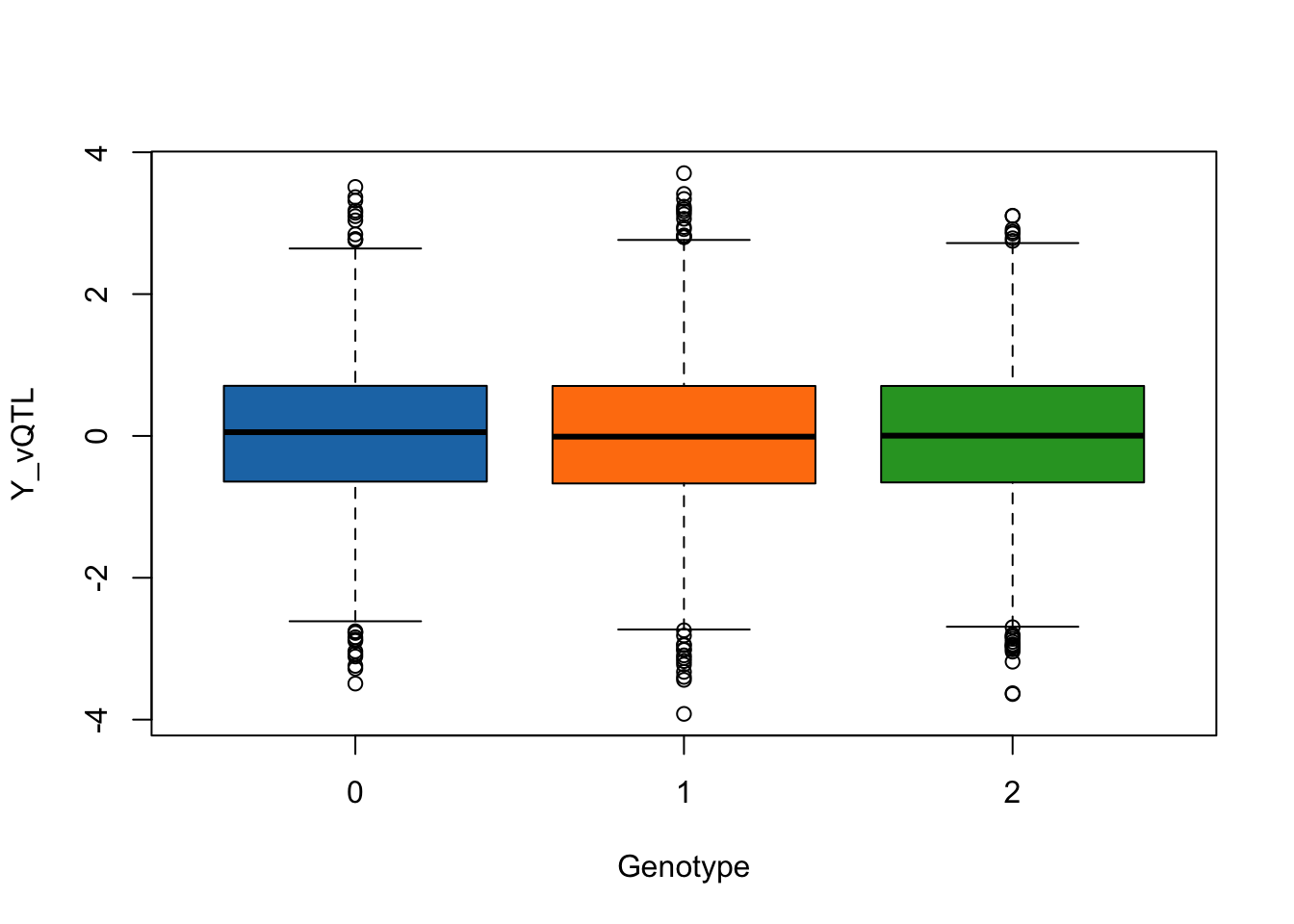

Version	Author	Date
5949e8a	Joelle Mbatchou	2025-06-10
648aef4	Joelle Mbatchou	2025-06-09

Testing for (mean) QTL

We use of lm() in R to assess phenotypic mean differences across genotypes for each variant.

Copy/Run the following command to enable the lm_test function in your current R environment.

# This function applies linear regression test to each of the simulated variant for a given trait
# trait_name = {"Y_vQTL", "Y_gxe"}
lm_test <- function(data, trait_name) {
  
  p_values <- rep(NA, n_snps)
  names(p_values) <- colnames(data$genotype)

  for(i in 1:n_snps){
    p_values[i] <- summary(lm(phenotype[, trait_name] ~ genotype[,i], data = data))$coef[2,4]
  }
  
  # Return the p-values
  return(p_values)
}

Based on the parameters used in the simulation, would we expect significant result when testing the causal SNP1?

First we do it for trait “Y_vQTL” (do it again on your own for the other trait “Y_gxe”)

trait_name <- "Y_vQTL"
qtl_pvals <- lm_test(data = simulated_data, trait_name =  trait_name)

qtl_pvals[1] # P-value of the causal SNP1

     SNP1 
0.2942319

You can make a qq plot to visualize the p-values highlighting the causal SNP1.

Copy/Run the following command to enable the plot_qq function in your current R environment.

plot_qq <- function(pvals){
  qq(pvals)
  points(-log10(ppoints(n_snps)[rank(pvals)[1]]), -log10(pvals[1]),
       col = "blue", pch = 19, cex = 1.5)
}

plot_qq(qtl_pvals)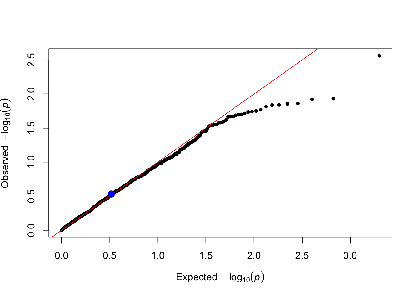

Version	Author	Date
5949e8a	Joelle Mbatchou	2025-06-10

Testing for vQTL

We make use of Levene’s test to assess phenotypic variance differences across genotypes for each variant.

Copy/Run the following command to enable the levene_test function in your current R environment.

# This function applies levene test to each of the simulated variant for a given trait
# trait_name = {"Y_vQTL", "Y_gxe"}
levene_test <- function(data, trait_name) {
  
  p_values <- rep(NA, n_snps)
  names(p_values) <- colnames(data$genotype)
  
  for(i in 1:n_snps){
    # Ensure the genotype is a factor
    factor_geno <- as.factor(data$genotype[,i])
  
    # Calculate the absolute deviations from the group means
    abs_dev <- abs(data$phenotype[, trait_name] - ave(data$phenotype[, trait_name], factor_geno, FUN = mean))

    # Perform an ANOVA on the absolute deviations
    p_values[i] <- summary(aov(abs_dev ~ factor_geno))[[1]]$`Pr(>F)`[1]
  }
  
  # Return the p-values
  return(p_values)
}

Based on the parameters used in the simulation, would we expect significant result when testing the causal SNP1?

trait_name <- "Y_vQTL"
levene_pvals <- levene_test(data = simulated_data, trait_name =  trait_name)  # Levene's test for variance differences

levene_pvals[1] # P-value of the causal SNP1

     SNP1 
0.2343523

You can make a qq plot to visualize the p-values highlighting the causal SNP1.

plot_qq(levene_pvals)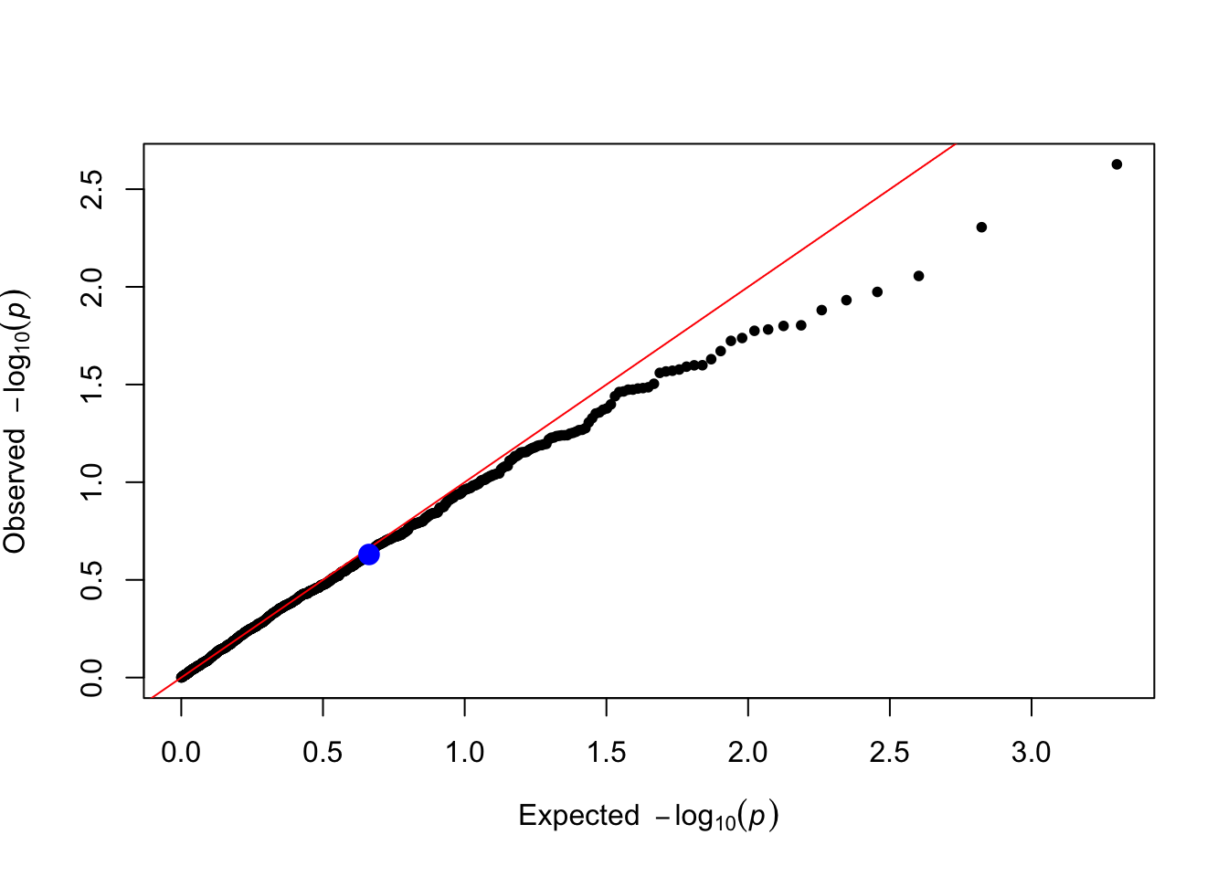

Version	Author	Date
5949e8a	Joelle Mbatchou	2025-06-10

Testing for GxE

We again use of lm() in R but this time also include an interaction term with the environment.

Copy/Run the following command to enable the gxe_test function in your current R environment.

gxe_test <- function(data, trait_name){
  pvals <- rep(NA, n_snps)
  names(pvals) <- colnames(data$genotype)

  for(i in 1:n_snps){
    pvals[i] <- summary(lm(phenotype[, trait_name] ~ genotype[,i]*covariate$environment, data = data))$coef[4,4]
  }
  
  return(pvals)
}

trait_name <- "Y_vQTL"
gxe_pvals <- gxe_test(data = simulated_data, trait_name =  trait_name)
gxe_pvals[1] # P-value of the causal SNP1

     SNP1 
0.4361276

You can make a qq plot to visualize the p-values highlighting the causal SNP1.

plot_qq(gxe_pvals)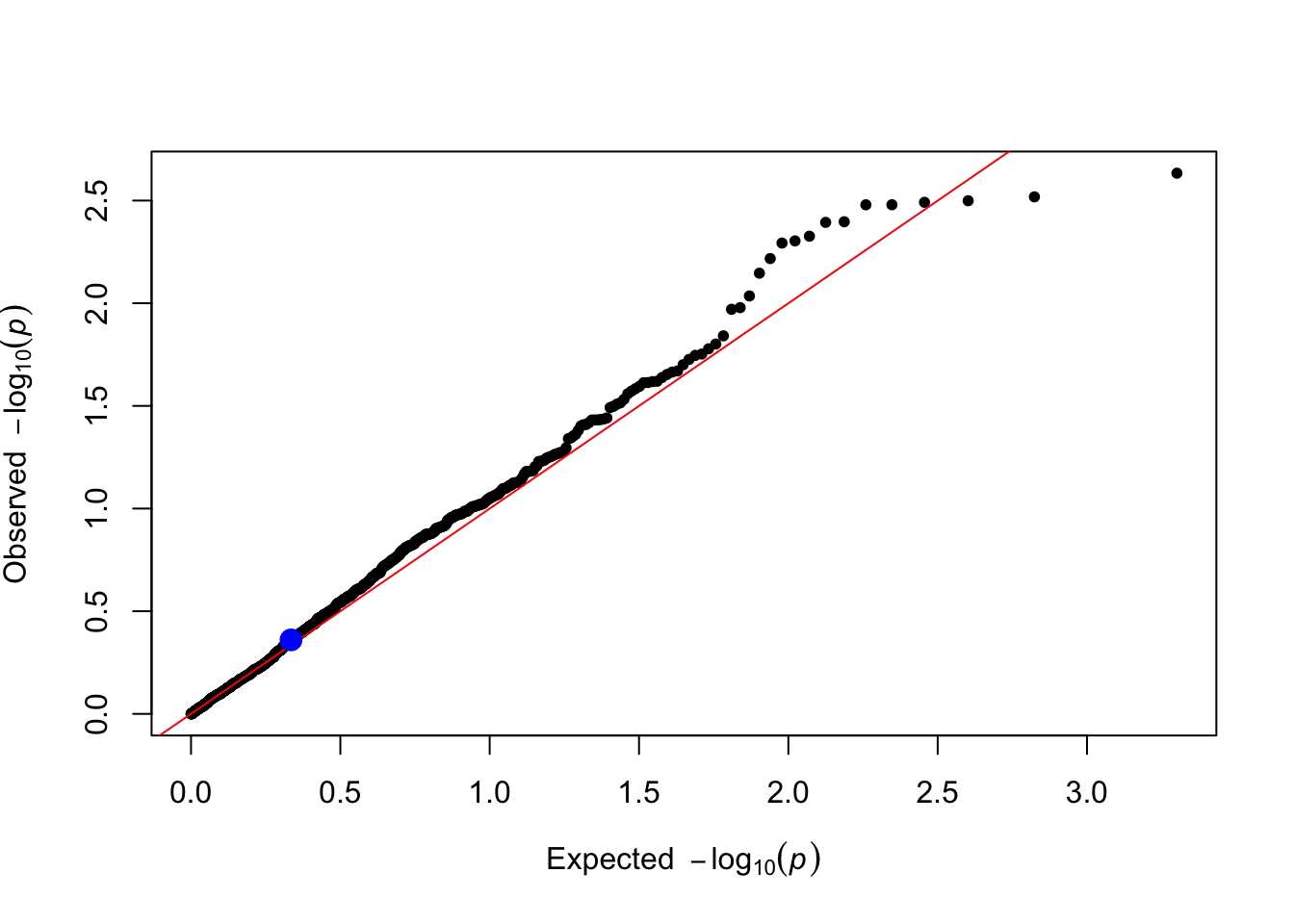

Version	Author	Date
5949e8a	Joelle Mbatchou	2025-06-10

Exploration across scenarios

Modify mean_effect and variance_effect to simulate different scenarios:

SNP1 affects only the mean (variance_effect = 0).

simulated_data <- simulate_vqtl_data(mean_effect = 0.1, variance_effect = 0)
trait_name <- "Y_vQTL"
boxplot(phenotype[,trait_name] ~ genotype[,"SNP1"], data = simulated_data,
        xlab = "Genotype",
        ylab = trait_name,
        col = c("#1f77b4", "#ff7f0e", "#2ca02c"))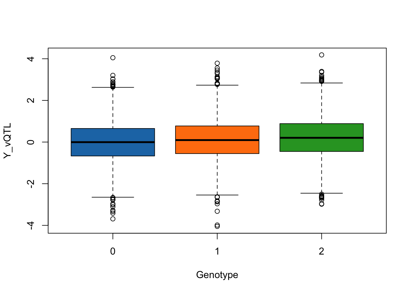

Version	Author	Date
5949e8a	Joelle Mbatchou	2025-06-10

qtl_pvals <- lm_test(data = simulated_data, trait_name =  trait_name)
plot_qq(qtl_pvals)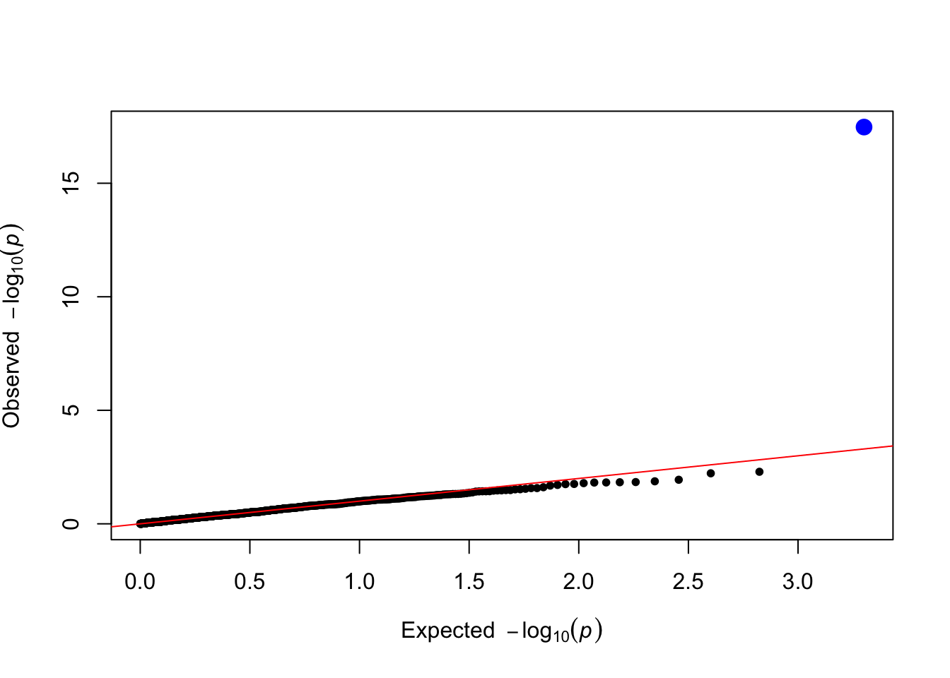

Version	Author	Date
5949e8a	Joelle Mbatchou	2025-06-10

levene_pvals <- levene_test(data = simulated_data, trait_name =  trait_name)
plot_qq(levene_pvals)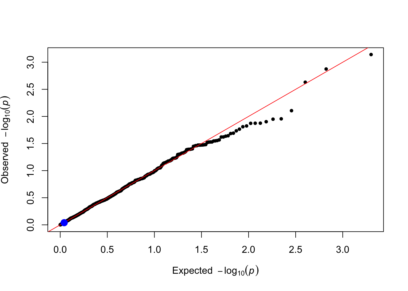

Version	Author	Date
5949e8a	Joelle Mbatchou	2025-06-10

gxe_pvals <- gxe_test(data = simulated_data, trait_name =  trait_name)
plot_qq(gxe_pvals)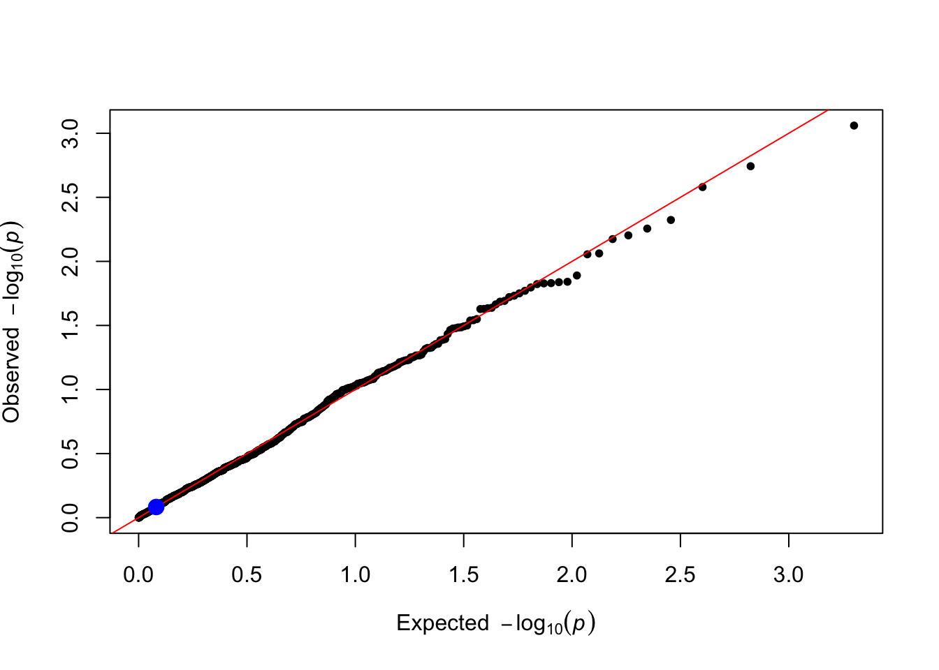

Version	Author	Date
5949e8a	Joelle Mbatchou	2025-06-10

SNP1 affects only the variance (mean_effect = 0).

simulated_data <- simulate_vqtl_data(mean_effect = 0, variance_effect = 0.1)
trait_name <- "Y_vQTL"
boxplot(phenotype[,trait_name] ~ genotype[,"SNP1"], data = simulated_data,
        xlab = "Genotype",
        ylab = trait_name,
        col = c("#1f77b4", "#ff7f0e", "#2ca02c"))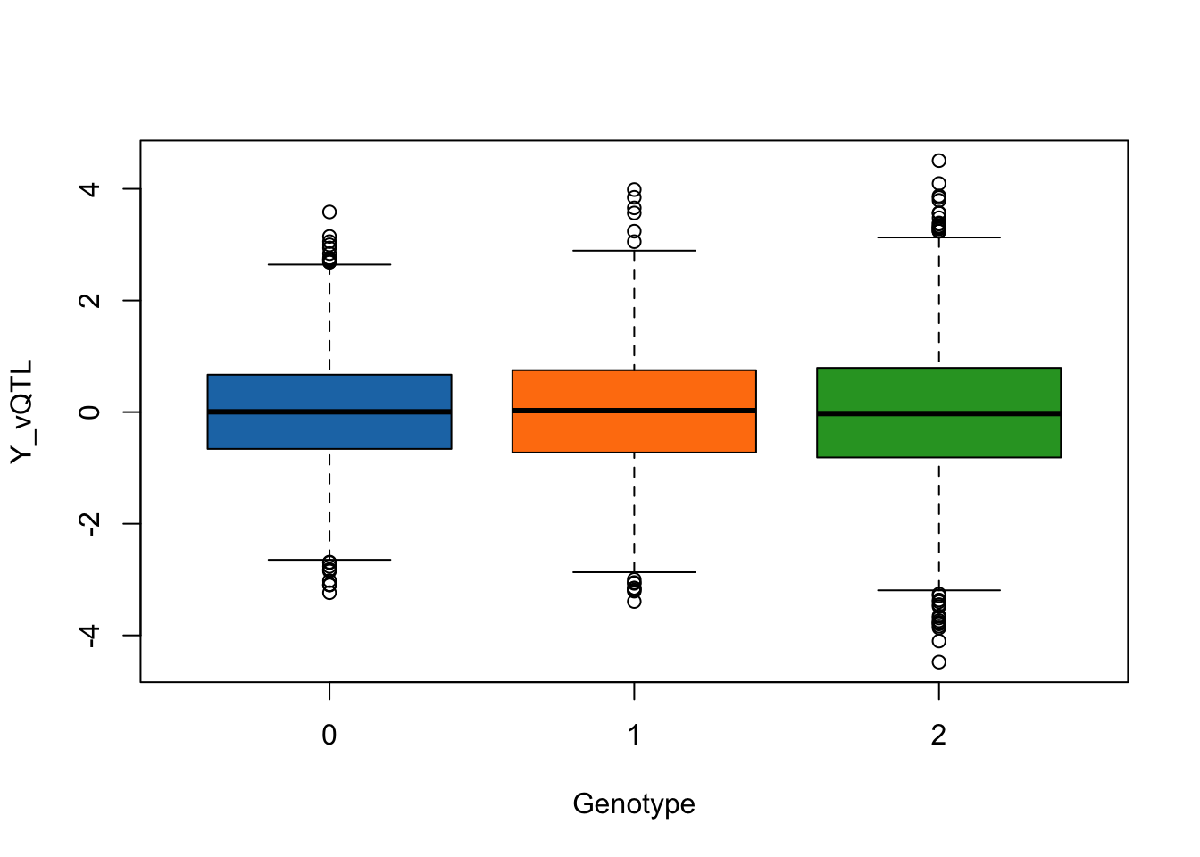

Version	Author	Date
5949e8a	Joelle Mbatchou	2025-06-10

qtl_pvals <- lm_test(data = simulated_data, trait_name =  trait_name)
plot_qq(qtl_pvals)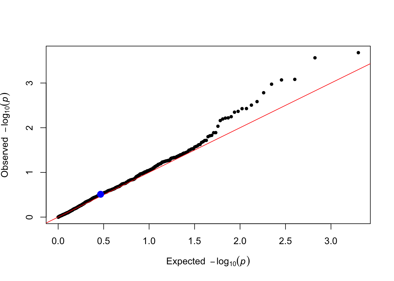

Version	Author	Date
5949e8a	Joelle Mbatchou	2025-06-10

levene_pvals <- levene_test(data = simulated_data, trait_name =  trait_name)
plot_qq(levene_pvals)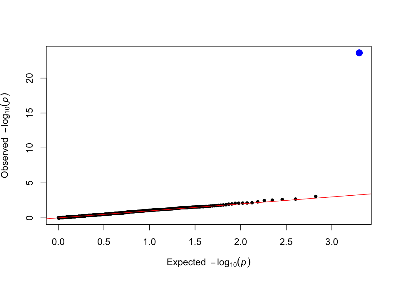

Version	Author	Date
5949e8a	Joelle Mbatchou	2025-06-10

gxe_pvals <- gxe_test(data = simulated_data, trait_name =  trait_name)
plot_qq(gxe_pvals)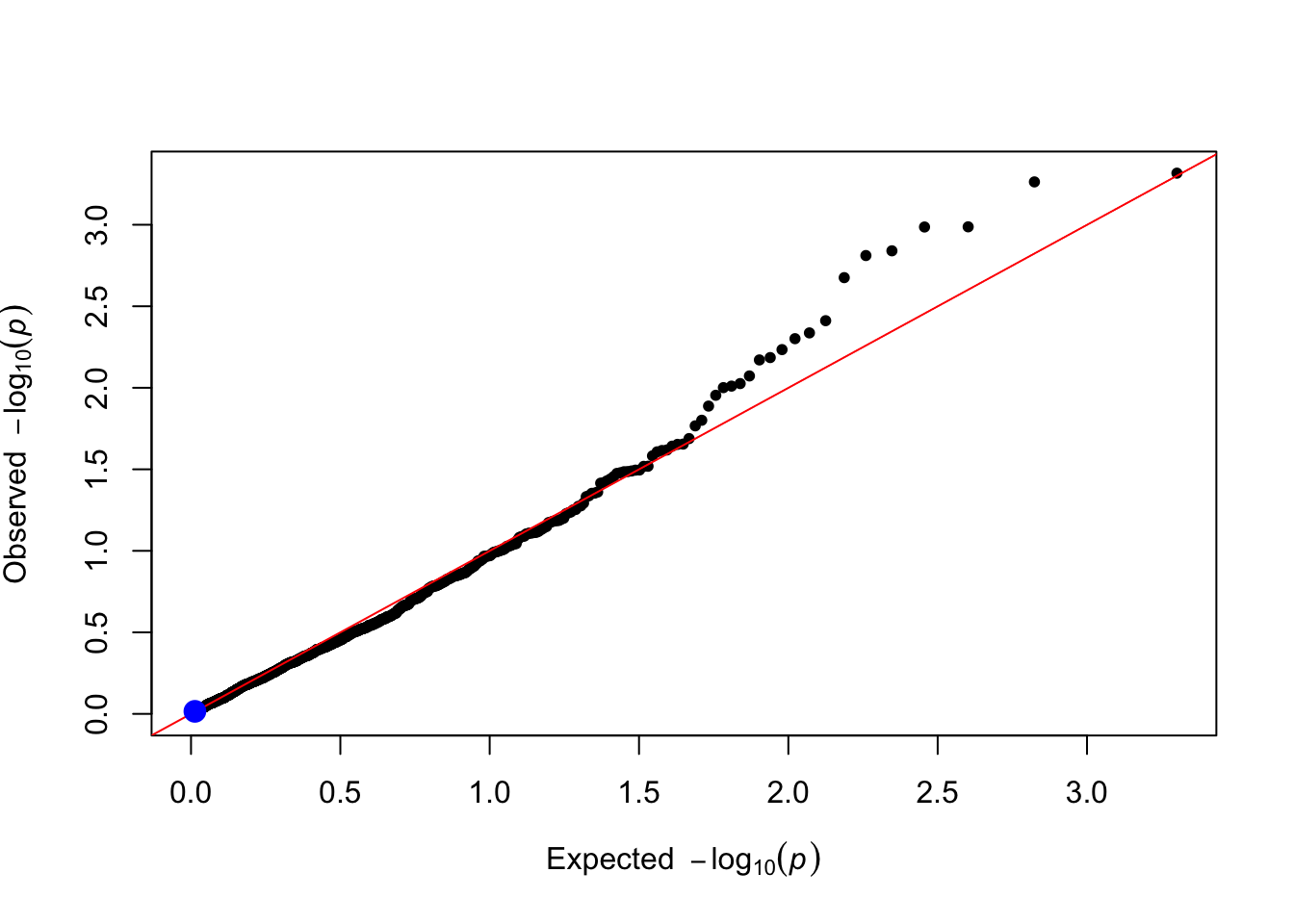

Version	Author	Date
5949e8a	Joelle Mbatchou	2025-06-10

SNP1 affects both the mean and variance.

simulated_data <- simulate_vqtl_data(mean_effect = 0.1, variance_effect = 0.2)
trait_name <- "Y_vQTL"
boxplot(phenotype[,trait_name] ~ genotype[,"SNP1"], data = simulated_data,
        xlab = "Genotype",
        ylab = trait_name,
        col = c("#1f77b4", "#ff7f0e", "#2ca02c"))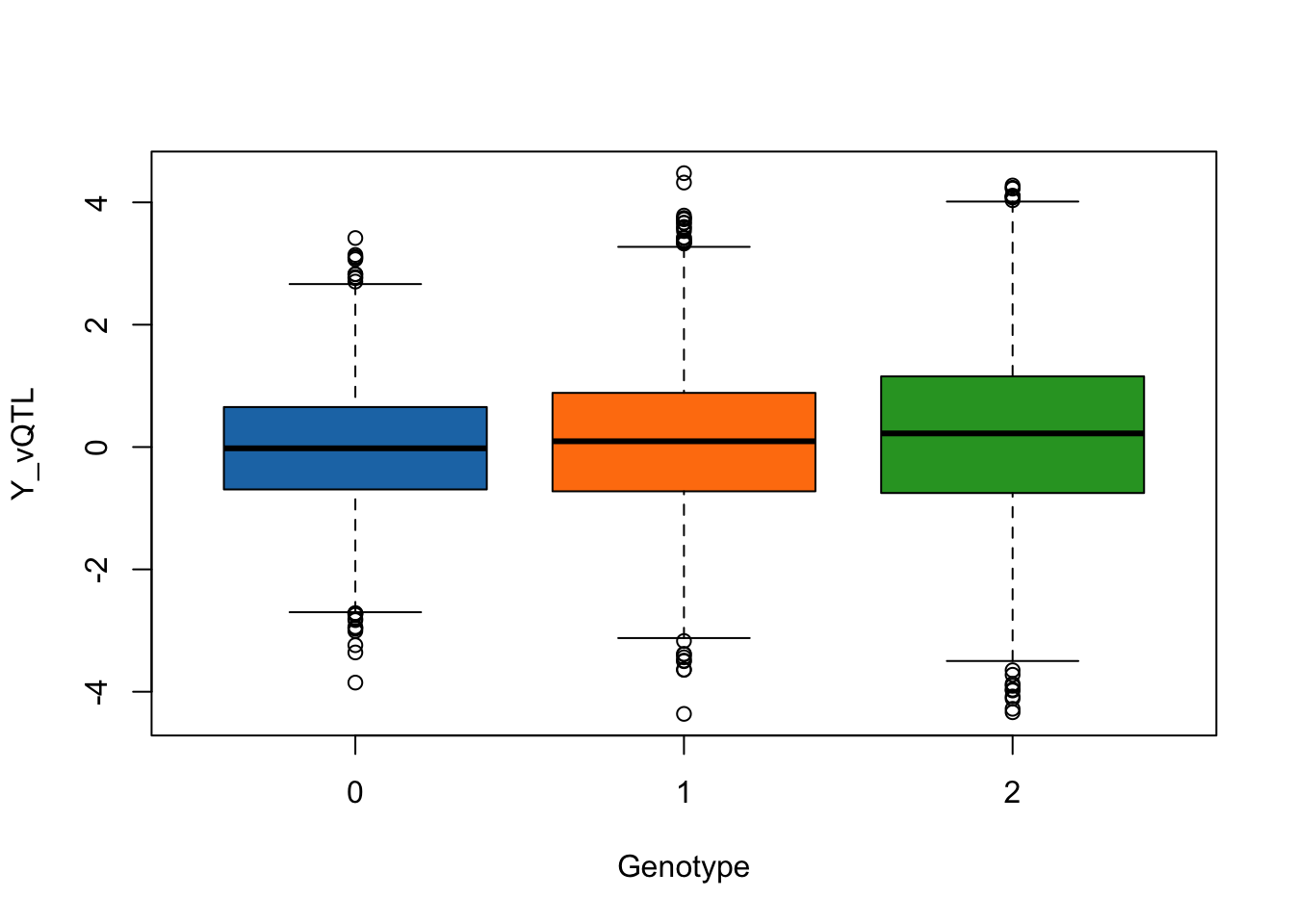

Version	Author	Date
5949e8a	Joelle Mbatchou	2025-06-10

qtl_pvals <- lm_test(data = simulated_data, trait_name =  trait_name)
plot_qq(qtl_pvals)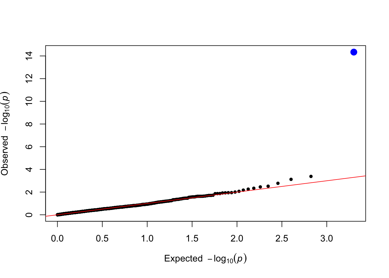

Version	Author	Date
5949e8a	Joelle Mbatchou	2025-06-10

levene_pvals <- levene_test(data = simulated_data, trait_name =  trait_name)
plot_qq(levene_pvals)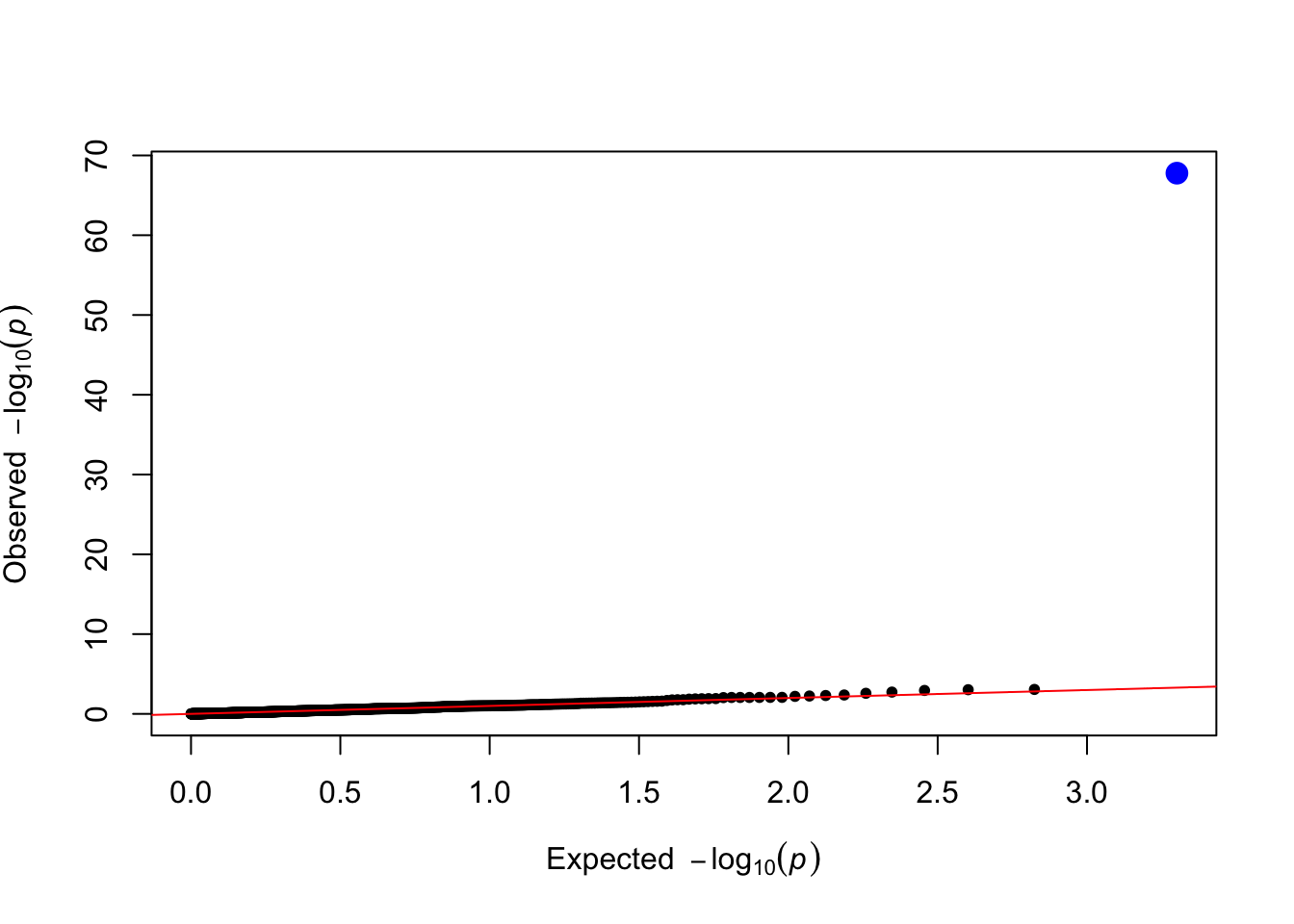

Version	Author	Date
5949e8a	Joelle Mbatchou	2025-06-10

gxe_pvals <- gxe_test(data = simulated_data, trait_name =  trait_name)
plot_qq(gxe_pvals)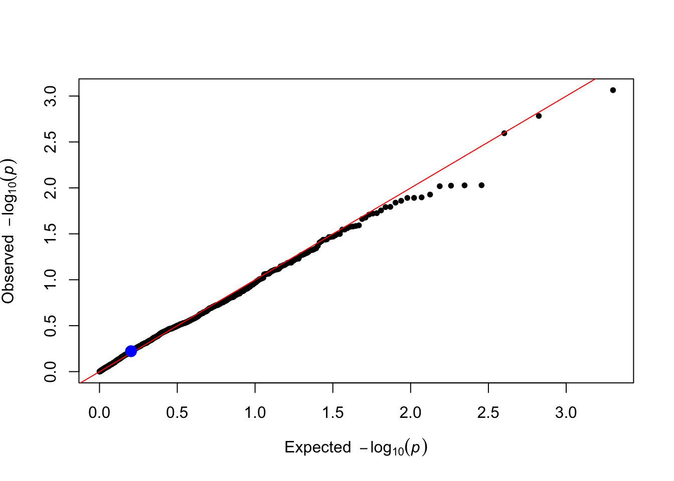

Version	Author	Date
5949e8a	Joelle Mbatchou	2025-06-10

gxe_pvals <- gxe_test(data = simulated_data, trait_name =  "Y_gxe")
plot_qq(gxe_pvals)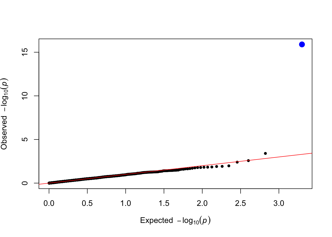

Version	Author	Date
5949e8a	Joelle Mbatchou	2025-06-10

sessionInfo()

R version 4.3.0 (2023-04-21)
Platform: aarch64-apple-darwin20 (64-bit)
Running under: macOS 14.7.4

Matrix products: default
BLAS:   /Library/Frameworks/R.framework/Versions/4.3-arm64/Resources/lib/libRblas.0.dylib 
LAPACK: /Library/Frameworks/R.framework/Versions/4.3-arm64/Resources/lib/libRlapack.dylib;  LAPACK version 3.11.0

locale:
[1] en_US.UTF-8/en_US.UTF-8/en_US.UTF-8/C/en_US.UTF-8/en_US.UTF-8

time zone: America/New_York
tzcode source: internal

attached base packages:
[1] stats     graphics  grDevices utils     datasets  methods   base     

other attached packages:
[1] qqman_0.1.8

loaded via a namespace (and not attached):
 [1] jsonlite_1.8.5   compiler_4.3.0   highr_0.10       promises_1.2.0.1
 [5] Rcpp_1.0.10      stringr_1.5.0    git2r_0.32.0     later_1.3.1     
 [9] jquerylib_0.1.4  yaml_2.3.7       fastmap_1.1.1    R6_2.5.1        
[13] workflowr_1.7.0  knitr_1.43       MASS_7.3-58.4    tibble_3.2.1    
[17] rprojroot_2.0.3  bslib_0.5.0      pillar_1.9.0     rlang_1.1.1     
[21] utf8_1.2.3       cachem_1.0.8     calibrate_1.7.7  stringi_1.7.12  
[25] httpuv_1.6.11    xfun_0.39        fs_1.6.2         sass_0.4.6      
[29] cli_3.6.1        magrittr_2.0.3   digest_0.6.31    rstudioapi_0.14 
[33] lifecycle_1.0.3  vctrs_0.6.2      evaluate_0.21    glue_1.6.2      
[37] whisker_0.4.1    fansi_1.0.4      rmarkdown_2.22   tools_4.3.0     
[41] pkgconfig_2.0.3  htmltools_0.5.5

Interaction testing and vQTL mapping

Summer Institute of Statical Genetics (Module QG3)

2025-06-10

Simulated dataset

Testing for (mean) QTL

Testing for vQTL

Testing for GxE

Exploration across scenarios