Solution for Practical 9: Within-family GWAS
Summer Institute of Statical Genetics (Module 15)
2023-07-26
Last updated: 2023-07-25
Checks: 7 0
Knit directory:
SISG2023_Association_Mapping/
This reproducible R Markdown analysis was created with workflowr (version 1.7.0). The Checks tab describes the reproducibility checks that were applied when the results were created. The Past versions tab lists the development history.
Great! Since the R Markdown file has been committed to the Git repository, you know the exact version of the code that produced these results.
Great job! The global environment was empty. Objects defined in the global environment can affect the analysis in your R Markdown file in unknown ways. For reproduciblity it’s best to always run the code in an empty environment.
The command set.seed(20230530) was run prior to running
the code in the R Markdown file. Setting a seed ensures that any results
that rely on randomness, e.g. subsampling or permutations, are
reproducible.
Great job! Recording the operating system, R version, and package versions is critical for reproducibility.
Nice! There were no cached chunks for this analysis, so you can be confident that you successfully produced the results during this run.
Great job! Using relative paths to the files within your workflowr project makes it easier to run your code on other machines.
Great! You are using Git for version control. Tracking code development and connecting the code version to the results is critical for reproducibility.
The results in this page were generated with repository version 4057e24. See the Past versions tab to see a history of the changes made to the R Markdown and HTML files.
Note that you need to be careful to ensure that all relevant files for
the analysis have been committed to Git prior to generating the results
(you can use wflow_publish or
wflow_git_commit). workflowr only checks the R Markdown
file, but you know if there are other scripts or data files that it
depends on. Below is the status of the Git repository when the results
were generated:
Untracked files:
    Untracked:  GWAS.ma
    Untracked:  causals.snplist
    Untracked:  ldRef.bed
    Untracked:  ldRef.bim
    Untracked:  ldRef.fam
    Untracked:  ldRef.log
    Untracked:  ldRef.map
    Untracked:  ldRef.ped
    Untracked:  test1.cma.cojo
    Untracked:  test1.jma.cojo
    Untracked:  test1.ldr.cojo
    Untracked:  test1.log
    Untracked:  test2.cma.cojo
    Untracked:  test2.jma.cojo
    Untracked:  test2.ldr.cojo
    Untracked:  test2.log
    Untracked:  test3.cma.cojo
    Untracked:  test3.jma.cojo
    Untracked:  test3.ldr.cojo
    Untracked:  test3.log
    Untracked:  test4.cma.cojo
    Untracked:  test4.jma.cojo
    Untracked:  test4.ldr.cojo
    Untracked:  test4.log
Note that any generated files, e.g. HTML, png, CSS, etc., are not included in this status report because it is ok for generated content to have uncommitted changes.
These are the previous versions of the repository in which changes were
made to the R Markdown (analysis/SISGM15_prac9Solution.Rmd)
and HTML (docs/SISGM15_prac9Solution.html) files. If you’ve
configured a remote Git repository (see ?wflow_git_remote),
click on the hyperlinks in the table below to view the files as they
were in that past version.
| File | Version | Author | Date | Message |
|---|---|---|---|---|
| Rmd | 4057e24 | Joelle Mbatchou | 2023-07-25 | edit |
This practical can be run in
R on your own computer.
This practical aims at illustrating that within-family GWAS are
robust to population stratification. We provide a set of R
commands below to simulate the phenotypes and genotypes (at \(M=1,000\) SNPs) of \(N=10,000\) independent sibling pairs. Each
sibling pair is sampled from \(g\)
subgroups, which differ in allele frequencies and mean phenotypes.
None of the \(M\) SNPs is associated with the trait within-each subpopulations. Therefore, the mean association \(\chi^2\) test statistic across SNPs is expected to equal 1. Any deviation reflects population stratification.
The R function CHISQ below returns the mean
association \(\chi^2\) test statistic
across \(M=1,000\) simulated SNPs for 3
analytical strategies:
simple linear regression using phenotypes and genotypes of the oldest siblings (
X1andY1)same as (1) but fitting 10 genotypic principal components (PC)
within-family GWAS from regressing
Y1-Y2onto colums ofX1-X2
Copy/Run the following command to enable the
CHISQ function in your current R
environment.
CHISQ <- function(N=10000,  # Sample size
                  M=1000,   # Number of SNPs tested
                  Fst=0.025,# Genetic differentiation between subgroups
                  vs=.05,   # variance explained by stratification
                  g=2,      # Number of subgroups
                  nPC=10){  # Number of PCs fitted
ms   <- rnorm(n=g,mean=0,sd=sqrt(vs))
p    <- runif(n=M,min=0.05,max=0.95)
tab  <- cut(1:N,breaks = quantile(1:N,probs = seq(0,1,len=g+1)),include.lowest = TRUE)
grp  <- as.numeric(tab)

simPS <- function(N,M,Fst,p,g){
  a    <- p*(1-Fst)/Fst
  b    <- (1-Fst)*(1-p)/Fst
  tab  <- cut(1:N,breaks = quantile(1:N,probs = seq(0,1,len=g+1)),include.lowest = TRUE)
  grp  <- as.numeric(tab)
  n    <- as.numeric(table(tab))
  X    <- do.call("rbind",lapply(1:g, function(k){
    px <- rbeta(M,shape1=a,shape2=b)
    do.call("cbind",lapply(1:M, function(j){
      rbinom(n=n[k],size=2,prob=px[j])
    }))
  }))
  return(X)
}

Xm  <- simPS(N,M,Fst,p,g) # Simulage genotypes of mother
Xf  <- simPS(N,M,Fst,p,g) # Simulate genotyoes of father

X1 <- do.call("cbind",lapply(1:M, function(j){
  rbinom(n=N,size=1,prob=Xm[,j]/2) + rbinom(n=N,size=1,prob=Xf[,j]/2)
}))

X2 <- do.call("cbind",lapply(1:M, function(j){
  rbinom(n=N,size=1,prob=Xm[,j]/2) + rbinom(n=N,size=1,prob=Xf[,j]/2)
}))

Y1 <- rnorm(n=N,mean=ms[grp],sd=sqrt(1-vs))
Y2 <- rnorm(n=N,mean=ms[grp],sd=sqrt(1-vs))

## PCA
SVD <- svd(scale(X1))
system.time( pcs <- SVD$u )

PC1 <- pcs[,1] * SVD$d[1]
PC2 <- pcs[,2] * SVD$d[2]
plot(PC1,PC2,pch=19,cex=0.5,col=grp,axes=FALSE,
     xlab="PC1",ylab="PC2")
axis(1);axis(2)
abline(h=0,v=0,col="grey")

## GWAS
gwas_pop <- do.call("rbind",lapply(1:M, function(j){
  summary(lm(Y1~X1[,j]))$coefficients[2,]
}))

gwas_pcs <- do.call("rbind",lapply(1:M, function(j){
  summary(lm(Y1~X1[,j] + pcs[,1:nPC]))$coefficients[2,]
}))

gwas_wf <- do.call("rbind",lapply(1:M, function(j){
  summary(lm(I(Y1-Y2)~I(X1[,j]-X2[,j])))$coefficients[2,]
}))

ChisqUnAdj  <- mean(gwas_pop[,3]^2)
ChisqPCAdj  <- mean(gwas_pcs[,3]^2)
ChisqQFAM   <- mean(gwas_wf[,3]^2)

return(c(UnAdj=ChisqUnAdj,PCAdj=ChisqPCAdj,QFAM=ChisqQFAM))
}
The CHISQ function has 5 input parameters:
N (sample size), M (number of SNPs tested),
Fst (a parameter measuring genetic differentiation between
subgroups in the sample), vs (variance explained by
stratification) and g (the number of subgroups in the
sample).
Let’s run a first sample with N=10000 individuals,
g=2 subgroups in the sample, M=1000 SNPs,
Fst=.025 and stratification explaining vs=.05
of the phenotypic variance.
set.seed(27072022)
system.time( testResults <- CHISQ(N=10000,M=1000,Fst=.025,vs=.05,g=2) )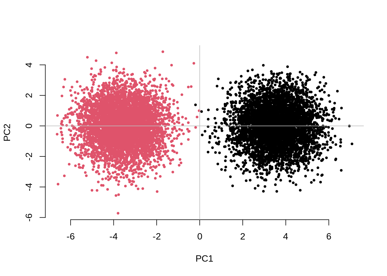
   user  system elapsed
 63.210   1.068  64.290
testResults UnAdj PCAdj QFAM
2.0576085 0.9916819 0.9163870 This example generates a PCA plot (PC1 vs PC2) showing a neat
separation between the two subgroups in the sample. In addition, the
mean association test statistic for the unadjusted analysis is
UnAdj~2.0, which indicates confounding due to population
stratification given that none of these SNPS are associated with the
phenotype. Note that the mean association test statistic is reduced to
PCAdj~1.0, when adjusting these analyses for 10 PCs and to
ChisqQFAM~0.9 for the within-family GWAS.
Question 1. Change the seed number (check the
set.seed() function above) and run the previous command
(CHISQ(N=10000,M=1000,Fst=.025,vs=.05,g=2)) in your own
environment. Do you find consistent observations?
set.seed(22061986)
system.time( testResults <- CHISQ(N=10000,M=1000,Fst=.025,vs=.05,g=2) )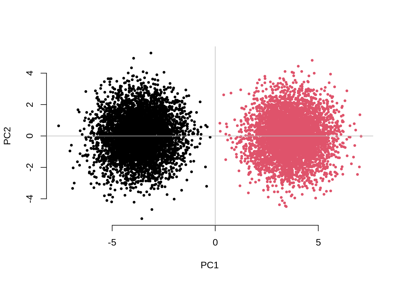
   user  system elapsed
 62.428   0.664  63.094
testResults UnAdj PCAdj QFAM
2.1654689 0.9471238 0.9442280 This examples takes about 1 minute to run.
Question 2. Increase the number of subgroups (e.g..
g=5, g=10, g=50). What can you
say about the separation between subgroups on the first two PCs? Is the
adjustment for 10 PCs still sufficient to control for inflation? If not,
how many PCs do you need to fit and why? What do you observe for the
within-family GWAS results?
CHISQ(N=10000,M=1000,Fst=.025,vs=.05,g=5,nPC=10)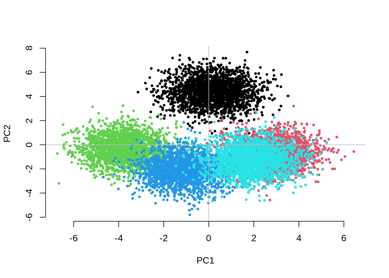
    UnAdj     PCAdj      QFAM
1.7859034 0.9903592 0.9410527
CHISQ(N=10000,M=1000,Fst=.025,vs=.05,g=10,nPC=10)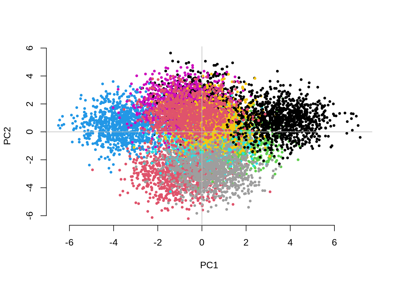
   UnAdj    PCAdj     QFAM
3.196399 1.048966 0.982059
CHISQ(N=10000,M=1000,Fst=.025,vs=.05,g=50,nPC=10)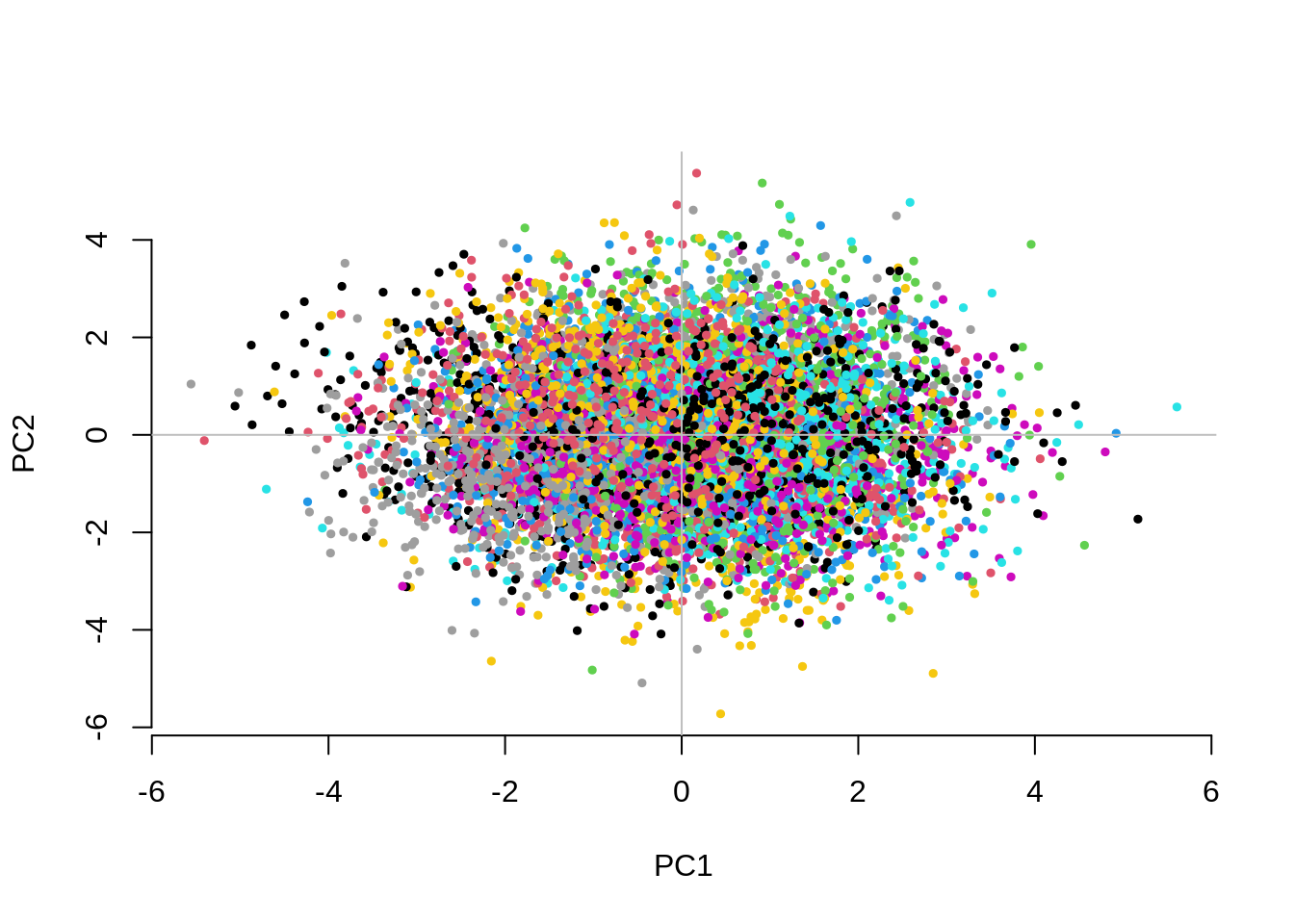
    UnAdj     PCAdj      QFAM
1.1605441 1.1258952 0.9512546
## Let's try fitting 50 PCs
CHISQ(N=10000,M=1000,Fst=.025,vs=.05,g=50,nPC=50)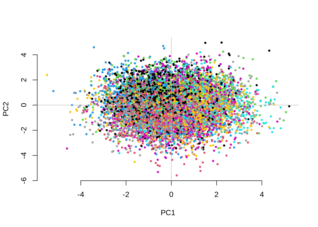
    UnAdj     PCAdj      QFAM
1.2320150 1.1311878 0.9845612
The separation between groups along the first two PCs decreases as we increase the number of groups. Fitting the 10 PCs seems to become inefficient. Fitting as many PCs as the number of groups seems to work but also substantially increases the computational time.
Question 3. Now set Fst=0.1 (that would
correspond to subgroups with different continental ancestries),
vs=0.1 and g=50. Are your conclusions from
Question 2 different?
CHISQ(N=10000,M=1000,Fst=.1,vs=.1,g=50,nPC=10)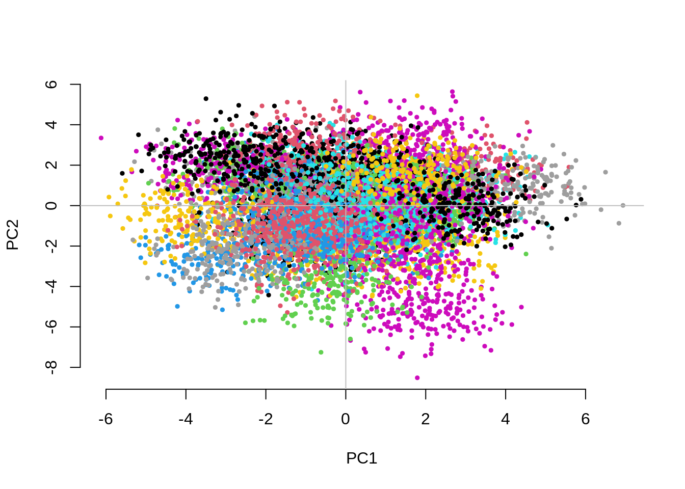
   UnAdj    PCAdj     QFAM
3.190113 2.474966 1.001763
CHISQ(N=10000,M=1000,Fst=.1,vs=.1,g=50,nPC=50)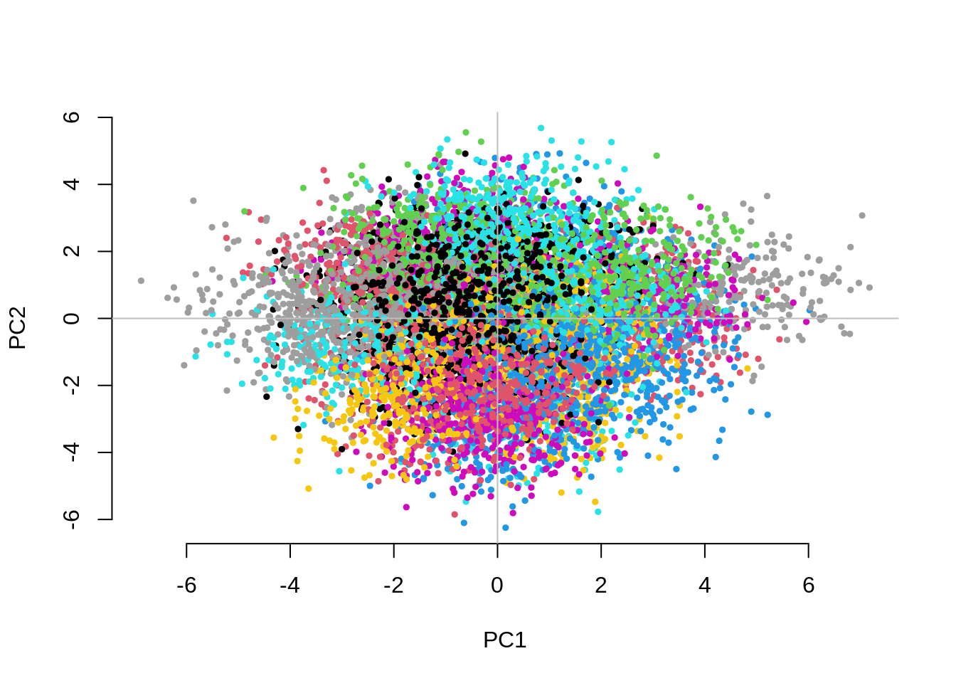
   UnAdj    PCAdj     QFAM
3.069871 1.057847 1.014468
sessionInfo()R version 4.3.1 (2023-06-16)
Platform: x86_64-pc-linux-gnu (64-bit)
Running under: Ubuntu 22.04.2 LTS
Matrix products: default
BLAS: /usr/lib/x86_64-linux-gnu/blas/libblas.so.3.10.0
LAPACK: /usr/lib/x86_64-linux-gnu/lapack/liblapack.so.3.10.0
locale:
[1] LC_CTYPE=C.UTF-8 LC_NUMERIC=C LC_TIME=C.UTF-8
[4] LC_COLLATE=C.UTF-8 LC_MONETARY=C.UTF-8 LC_MESSAGES=C.UTF-8
[7] LC_PAPER=C.UTF-8 LC_NAME=C LC_ADDRESS=C
[10] LC_TELEPHONE=C LC_MEASUREMENT=C.UTF-8 LC_IDENTIFICATION=C
time zone: Etc/UTC
tzcode source: system (glibc)
attached base packages:
[1] stats graphics grDevices utils datasets methods base
loaded via a namespace (and not attached):
[1] vctrs_0.6.3 cli_3.6.1 knitr_1.43 rlang_1.1.1
[5] xfun_0.39 highr_0.10 stringi_1.7.12 promises_1.2.0.1
[9] jsonlite_1.8.7 workflowr_1.7.0 glue_1.6.2 rprojroot_2.0.3
[13] git2r_0.32.0 htmltools_0.5.5 httpuv_1.6.11 sass_0.4.6
[17] fansi_1.0.4 rmarkdown_2.23 jquerylib_0.1.4 evaluate_0.21
[21] tibble_3.2.1 fastmap_1.1.1 yaml_2.3.7 lifecycle_1.0.3
[25] whisker_0.4.1 stringr_1.5.0 compiler_4.3.1 fs_1.6.2
[29] Rcpp_1.0.11 pkgconfig_2.0.3 rstudioapi_0.15.0 later_1.3.1
[33] digest_0.6.33 R6_2.5.1 utf8_1.2.3 pillar_1.9.0
[37] magrittr_2.0.3 bslib_0.5.0 tools_4.3.1 cachem_1.0.8